Widespread interest in understanding past, present, and future climate change and variability and the response and feedbacks of natural and managed ecosystems has motivated the development and application of models and techniques to provide climate data at relevant spatial and temporal scales. A wealth of observational data is available to support research over the historical record and geologic records provide indirect evidence of climate changes in the past. Quantitative estimates of paleo- and future climate (including atmospheric circulation as well as surface‑climate variables), however, must be obtained from climate models that account for the interactive changes in the global atmosphere and oceans that are driven by global boundary conditions, such as atmospheric trace‑gas concentrations and aerosols, earth-sun geometry, sea ice, sea level, and continental ice sheets. Simulations of global climate are conducted with general circulation models (GCMs), which are designed to balance model resolution and physics with computational requirements and limitations. Hence, long climate simulations (for example, centuries to millennia) have necessarily been run at relatively coarse spatial resolutions, which are on the order of a few degrees in latitude and longitude. GCMs are now being run for shorter time periods at finer resolution; however, the prevailing approach for obtaining finer spatial resolution climate information is to apply techniques for downscaling GCM output (for example, Maraun and others, 2010).
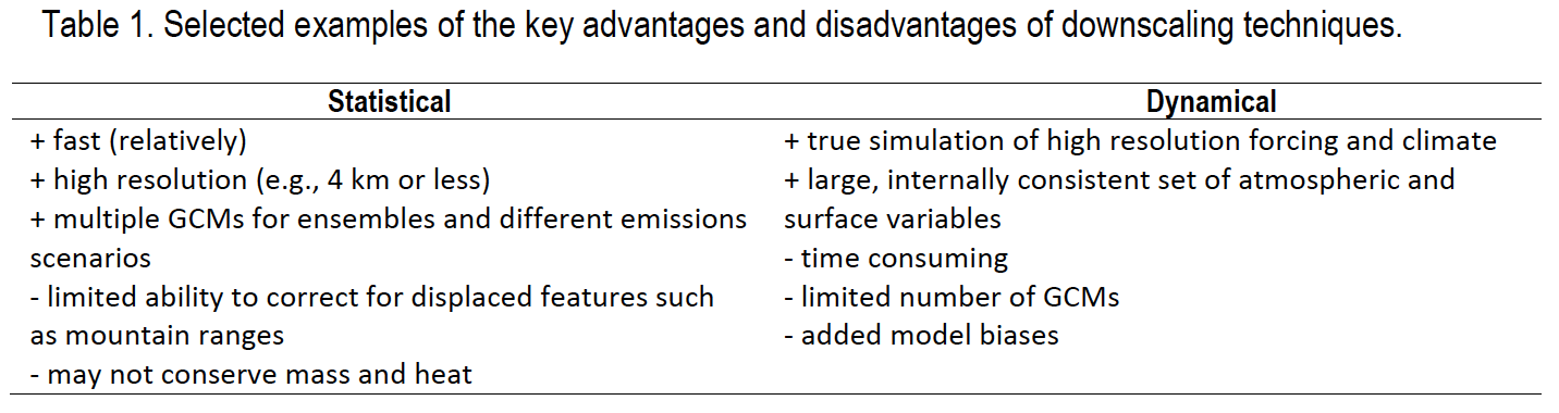
Downscaling techniques fall into two very different categories: statistical and dynamical. The techniques are complementary and both have strengths and weaknesses (table 1). Many variations of statistical downscaling exist, ranging in complexity from simple interpolation to application of statistical neural networks and weather generators. Wilby and others (2004) and references therein provide an excellent introduction to and overview of the techniques. All techniques are applied to downscale the climate (for example, temperature and precipitation) of a GCM grid cell (order of hundreds of kilometers in latitude and longitude) to a high resolution grid (order of ten kilometers or less). The high resolution grids are based on digital elevation models (DEMs) that represent more realistic topography than can be represented by low resolution GCMs.
Downscaling techniques can be relatively uncomplicated. For example, differences or anomalies between a future period and the present are calculated for each GCM grid cell, the anomalies are interpolated to a high resolution grid and the differences are added to observed climatology on the same high resolution grid (for example, Tabor and Williams, 2010). An additional computation is usually employed for precipitation to scale modeled values so the changes are essentially converted to percent change that is consistent with observed values. More complex techniques involve building statistical (for example, regression) relationships between observed climate fields and the grid cells of the DEM (for example, between 500 hPa heights and precipitation, Cayan and others, 2008). For temperature-related variables, the GCM data for the present and future are interpolated to the high resolution grid using these relationships and temperature lapse rate corrections. Various methods are used for distributing precipitation to reflect more realistic topography and to conserve the total precipitation from the GCM. The relatively smooth fields from the GCM are thus distributed to a grid that more realistically represents finer scale topography. There is limited ability to compensate for features in the GCM, such as orographic precipitation over mountainous regions that can be displaced geographically due to smoothed topography.
Dynamical downscaling or regional climate modeling (RCM) also relies on output from GCM simulations. Output from GCM simulations is used to derive time-varying (for example, 6-hour) lateral (vertical profiles of temperature, humidity, wind) and surface (pressure and sea surface temperature) boundary conditions for a three-dimensional model domain that is selected to capture the important synoptic- and mesoscale atmospheric circulation features that determine the climatology of a region of interest. The 6-hour boundary conditions are assimilated along the four edges and surface (ocean) of the model domain and the RCM then simulates atmospheric circulation and surface interactions internally. We illustrate “nesting” of an RCM in a GCM with maps of upper level pressure height and winds, sea level pressure and winds and surface temperature and precipitation for August 1996 (fig. 1).
The nesting technique provides a high level of fidelity between the synoptic‑scale GCM fields and the associated mesoscale resolution fields simulated by the RCM. The time sequence of the maps in this example illustrates the building of a blocking high pressure cell at 500 hPa and an associated heat-induced surface low pressure cell over the Great Basin, a common summertime feature. The associated temperature and precipitation maps display warm temperatures over the Great Basin and a well‑developed monsoon over the Southwest that extends into the inter-mountain West. At present, nesting of the RCMs within GCMs occurs only in one direction—from the GCM to the RCM—so there is no feedback between the models. Two-way nesting techniques, in which a GCM and an embedded RCM interact continuously, are being developed at a number of modeling centers. One-way nesting is potentially subject to mismatches between the simulated fields and those of the GCM along the exit or downwind boundary of the RCM. Such mismatches occur, for example, because the amount of water vapor or the wind speed in the RCM differs from that of the GCM, which can result in excessive precipitation along the boundary. For this reason, model domains are usually designed to be larger than the area of interest so that a number of grid cells can be trimmed away from the border to eliminate boundary artifacts.
To a large extent, the climate variability of the driving GCM determines the variability of the climate produced by the RCM. Although regional climate models in general can improve on the details of GCM simulations through dynamical downscaling over complex terrain, they cannot, for example, improve upon or make substantial changes to features of the large-scale circulation or SSTs produced by a GCM. This means that, for example, if the jet stream is incorrectly placed in a GCM, it also will be incorrectly placed in the RCM. Regional climate simulations thus reflect not only model-to-model differences among the driving GCMs but also added internal biases related to parameterization of physical processes (for example, cloud formation) and other factors. It is known, for example, that the choice of the numerical scheme that is used in RegCM3 to simulate convective precipitation influences other fields, such as air temperature.