To provide some background that is relevant to coupling GCMs with RCMs, we provide a brief overview and comparison of a representative group of GCMs that were used in the CMIP and IPCC AR4, including the models used for our regional climate simulations. We focus on summarizing simulated surface temperature and precipitation because these variables can be readily compared with observations and because the degree of agreement with observations and among the models is an indication of how biases in the GCM atmospheric circulation and sea surface temperatures may influence associated RCM simulations.
All GCMs are designed to simulate the dynamics and processes of the atmosphere and ocean; however, the models can differ in how the processes are represented or parameterized, the numerical methods used to solve model equations, the horizontal and vertical resolution at which the models are run and how the atmospheric and ocean models interact. These model-to-model differences translate into differences in the sensitivity of the individual models to changes in forcing (for example, volcanic eruptions and atmospheric trace-gas concentrations) and in their simulated climatologies.
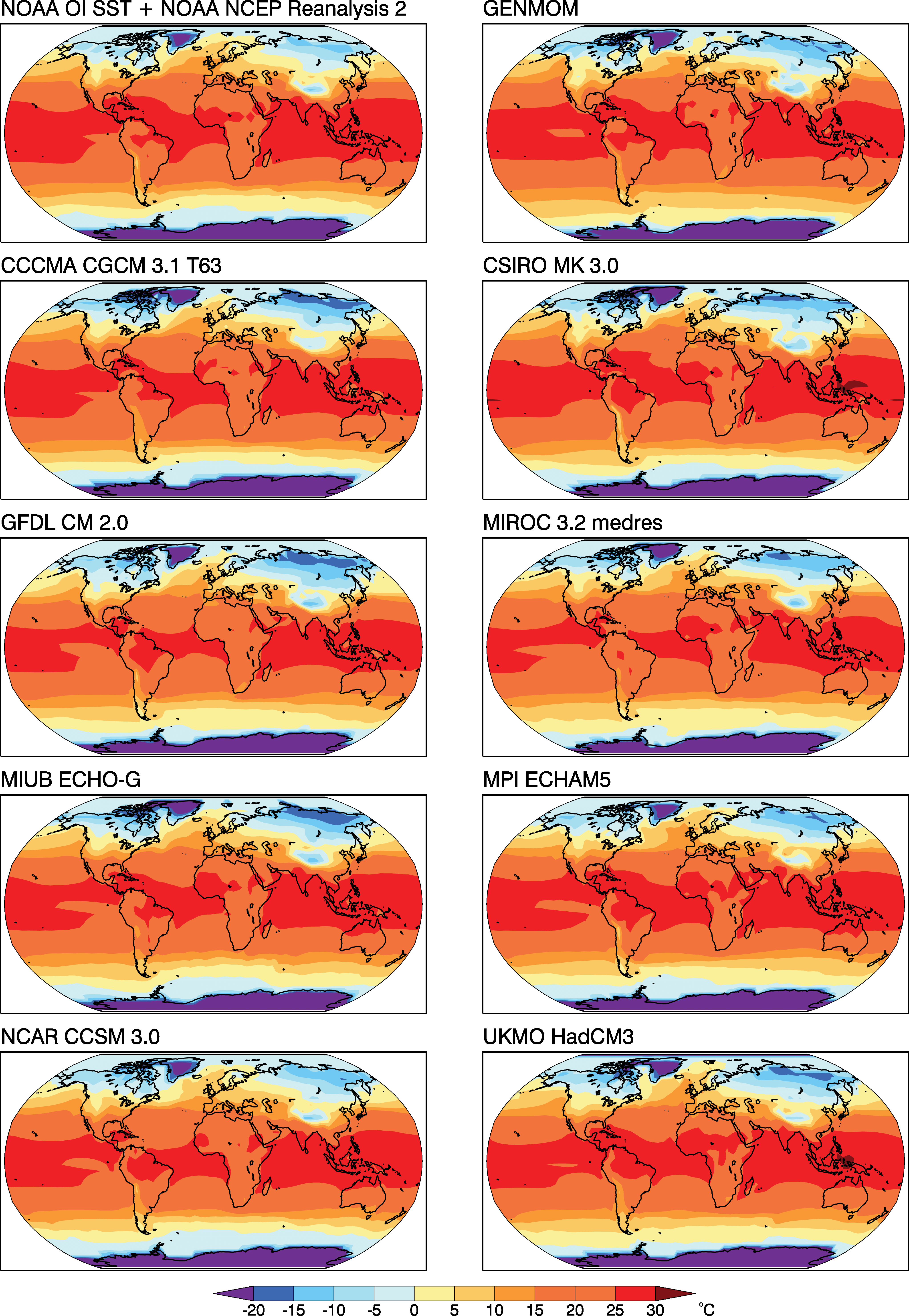
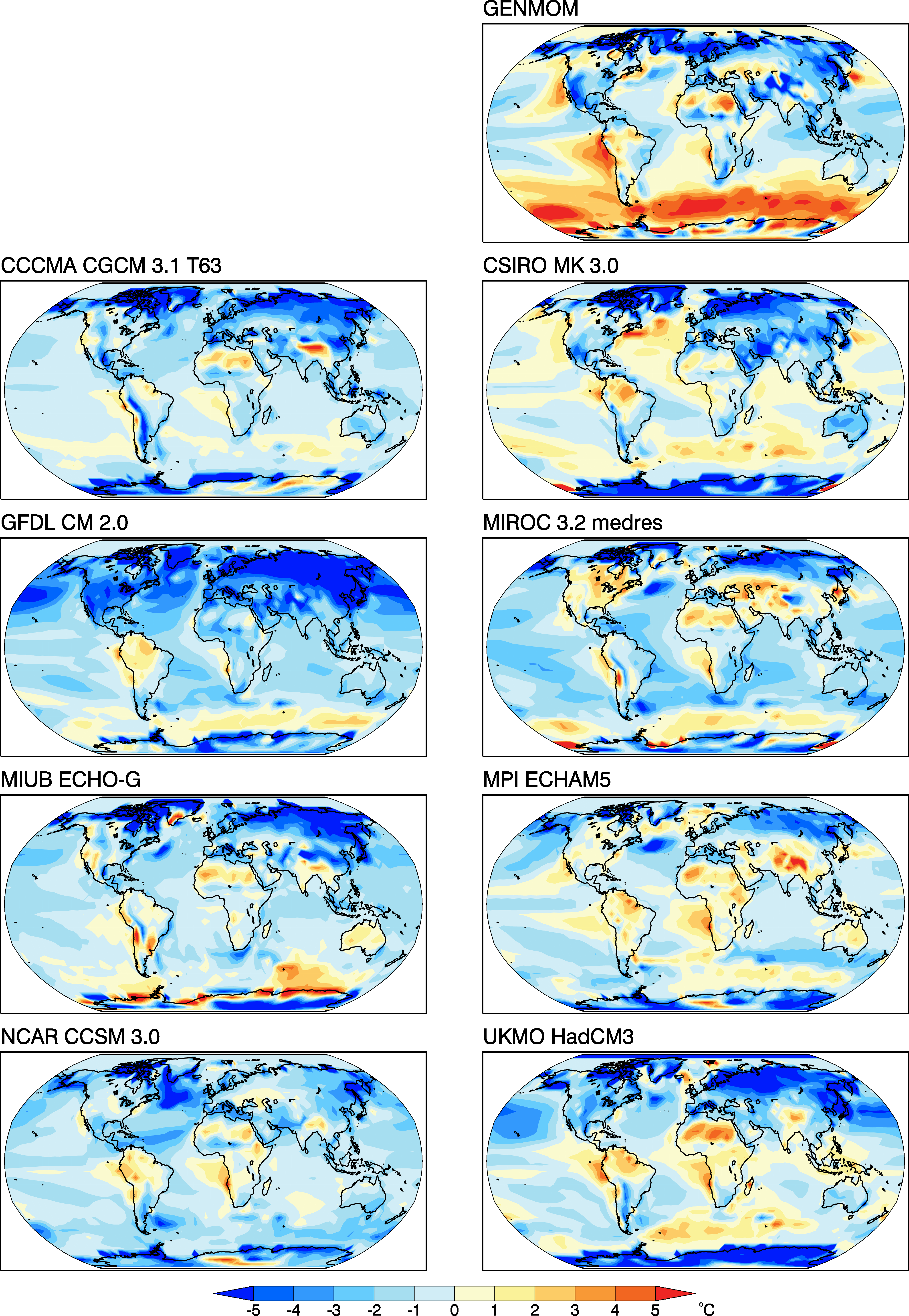
The global distribution and gradients of mean-annual air temperature climatology simulated by the IPCC GCMs compare well both with observations and among the models (fig. 4). Relative to observations, model‑dependent cold biases are evident over the Northern Hemisphere with a range of cold and warm bias over North America (fig. 5). The GFDL CM2.0 and GENMOM simulations display cold biases over North America of several degrees or more on an annually averaged basis.
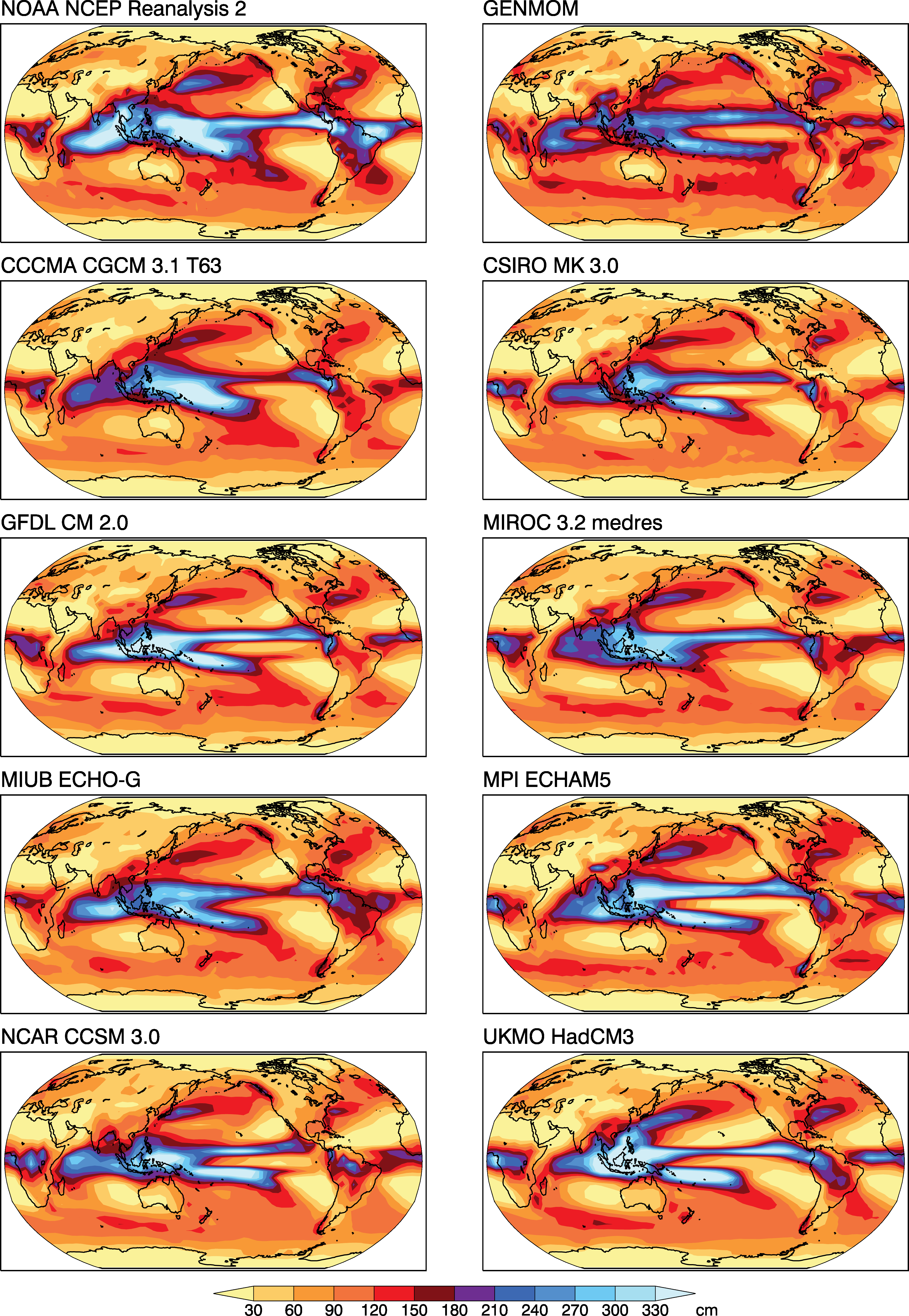
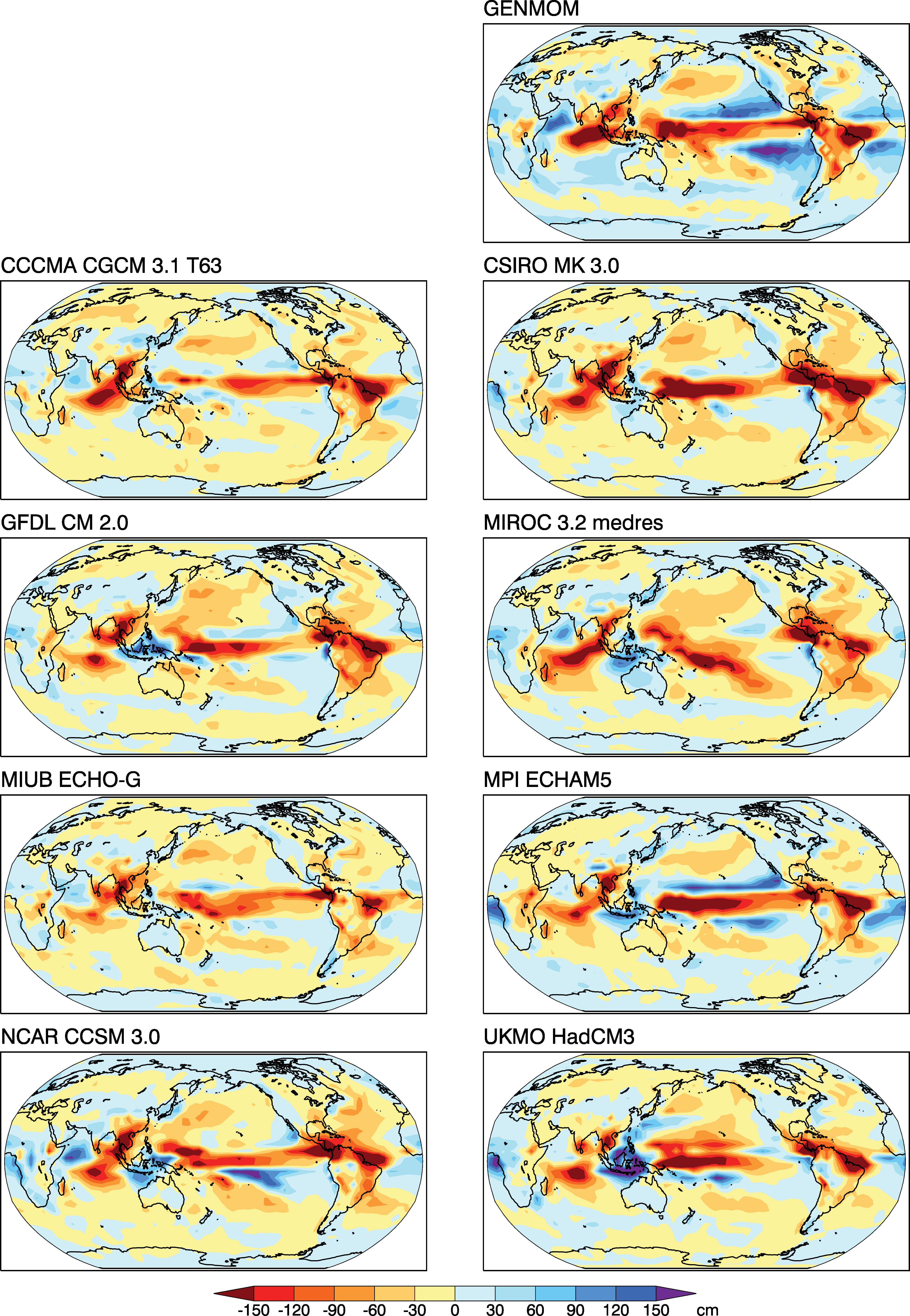
Climate models simulate both dynamic precipitation (for example, wintertime storms moving off the North Pacific Ocean into the Pacific Northwest) and convective precipitation (for example, thunderstorms, the monsoon over the Southwest). The physics and the temporal and spatial characteristics of precipitation are complex. Improving the ability of models to simulate precipitation remains a major challenge and goal for climate modelers. The global patterns and gradients of precipitation are captured by the models, but not as well as those of air temperature (fig. 6). The observed precipitation maximum in the equatorial region is reproduced in general by the models, but the magnitude and distribution of the maxima vary considerably with respect to observations and among the models (fig. 7). Most of the models tend to produce too much precipitation over Western North America and too little over Eastern North America. This pattern is associated with sea surface temperatures and the mid- to high-latitude atmospheric circulation. The wet bias in GFDL CM2.0 and GENMOM precipitation over Western North America coincides with the cold bias discussed above.
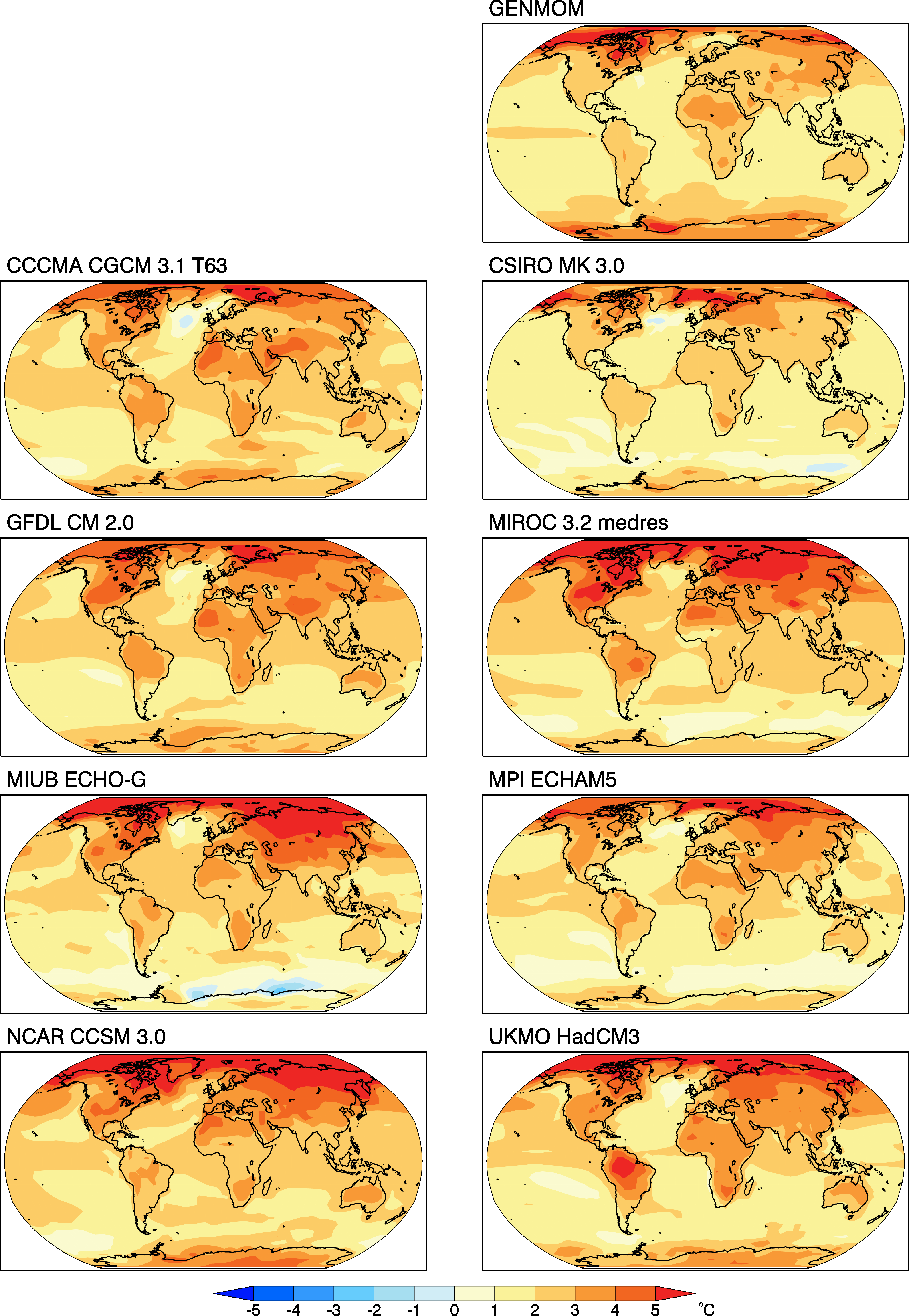
A fundamental metric that is used to characterize climate models is their sensitivity to a doubling of atmospheric CO2 (2XCO2) concentrations. The average, global temperature sensitivity of the GCMs that are included in the IPCC AR4 is ~3oC, with a range of 2–4.5oC. The temperature patterns simulated by models generally are similar globally (fig. 8). High‑latitude warming (that is, “polar amplification”) is a common feature in all simulations, as is a larger response of land as opposed to ocean temperatures. Regionally, the sensitivity of the models can differ by up to a few degrees (fig. 8). Although the general agreement among the models is remarkably good at the global scale, such regional difference in their sensitivity is a factor in determining temperature response changes at the regional scale. Over North America, the GCMs used to drive the RegCM3 display a range of sensitivities of 2–3oC (GENMOM), 2–4oC (ECHAM5), and 3–5oC (GFDL CM2.0).