This example demonstrates some basic techniques for how to download and manipulate monthly climate data. The data are downloaded in NetCDF format from the Regional Climate Downloader (RCD) application and we use the Interactive Data Language (IDL) programming language (see disclaimer) to create annual averages of the monthly data and the IDL graphics routines to plot the averages. If you are not familiar with RCD please see the tutorial first. Although the code is specific to IDL, the overall process should be similar in other analysis packages. The full sample code used in this example can be found here.
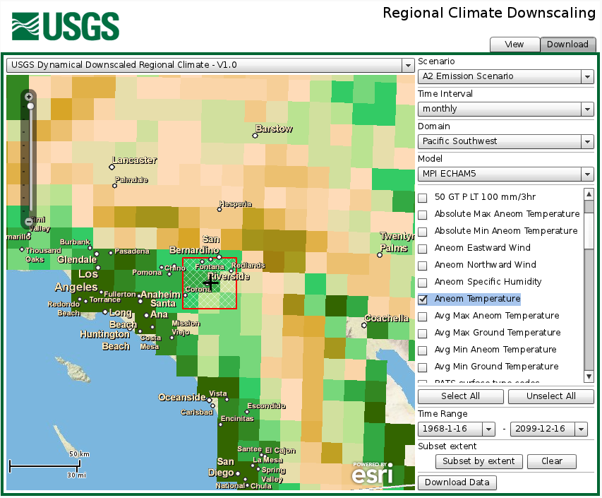
Step 1: Use the RCD application to zoom into Riverside, CA and then use the “Subset extent” tool (click on the “Subset by extent” button) to draw a box for the 9 grid cells surrounding Riverside. Each grid cell is 15 km by 15 km, so the downloaded values will be the average of the surrounding 9 grid cells which cover about 2025 square kilometers (about 780 square miles). Note that the grid cells are the smallest unit of area and thus data for the simulations; selecting a point by latitude and longitude will select the grid cell containing the point and the data will be the average for that grid cell. Averaging over a number of grid cells ensures that our results do not depend on one model grid cell; although, a single grid cell could be of interest for some applications.
Use the controls on the right to select Aneom Temperature and download the files for each of the four models (NOAA NCEP, MPI ECHAM5, USGS GENMOM, and GFDL CM2.0). The Aneom Temperature is the 2-meter air temperature (detailed description of all the model variables are given in the variable metadata). Rename the downloaded time series files as Riverside_NCEP.nc, Riverside_ECH5.nc, Riverside_GENMOM.nc, and Riverside_GFDL.nc, respectively.
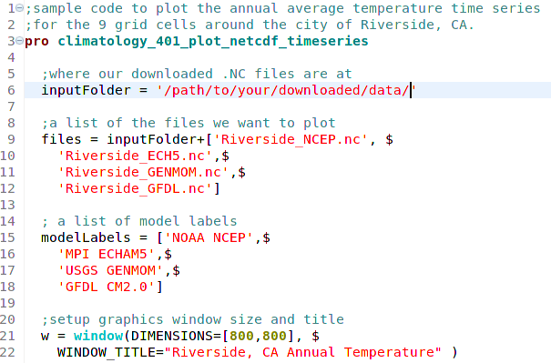
Step 2: The first 22 lines of code above 1) identify the folder where you saved your files (line 6), 2) list the names of the files to be used (lines 9-12), 3) specify title for the respective climate models (lines 15-18) and 4) set the size of the graphics window that will be opened by IDL (lines 21-22). The various text colors are IDL conventions and the lines that begin with a “;” are comments.

Step 3: A FOR structure is used to iterate over each file, average the data and plot the average:
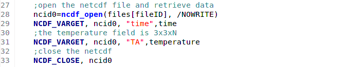
Step 4: Within the FOR loop the current NetCDF file is opened (line 28) and the monthly dates and air temperature values are read from the file (lines 29 and 31). The NetCDF file is then closed (line 33). The temperature variable is a 3‑dimensional array of size 3x3xN, where N is the number of months which differs depending on the model data being read. In the NCEP file N is 516 months, representing 43 years (1968-2010) of data. The 3×3 dimensions of the array store the 9 cells we downloaded in Step 1 using the RCD application.
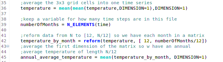
Step 5: In line 36, the 9 cells surrounding Riverside, CA are averaged into a single number. The resulting temperature variable is now a 1-dimensional vector of N averages. Line 39 is a dynamic way to determine how many months are in the current file (N). Line 42 may be a little confusing at first if you are not familiar with mathematical programming packages such as IDL or MATLAB. The code in Line 42 “reforms” the temperature variable from a 1-dimensional array of length N into a 2-dimensional array of size 12 x N/12. This reformatting associates the months (1-12) with the first dimension and all the years (N years divided by 12 months) to second dimension, and provides an efficient way to create an annual average (line 45).
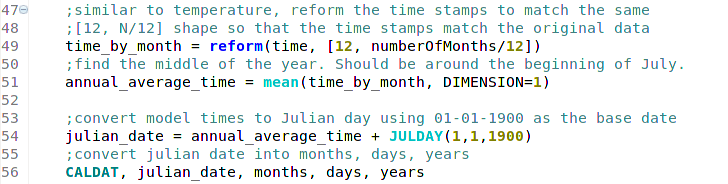
Step 6: The code in lines 49 and 51 does essentially the same thing with time that we did with air temperature in lines 42 and 45. This is step is needed to ensure our temperature and time variables both have the same “shape”, that is, so the temperatures correspond to the correct month.
Following standard NetCDF conventions, the time variable is recorded as the number of days since 01-01-1900. To be a more intuitive, we convert this value into Julian days (line 54), which is converted into days, months, and years. Each of these time stamp arrays will be the same length as the annual_average_temperature variable.
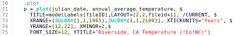
Step 7: Now that we have the annual_average_temperature and the corresponding Julian dates, we can plot the temperature time series. Because the code is in an interative FOR loop (line 25), four plots, one for each model, will be made in the open IDL window (below). In the code that does the plotting, (lines 70-74), we use a number of IDL keywords: the TITLE keyword is set to the model labels defined in lines 15-18., the LAYOUT keyword defines where in the graphics window the current plot should be placed, and the /CURRENT keyword is set to so that all the plots are made in the same IDL graphics window. The XRANGE keyword sets the x-axes range to 1-1-1965 through 1-1-2100, and the XTICKUNITS keyword set to “Years” so that IDL will label the Julian dates in year notation. The YRANGE keyword forces the y-axes for all the plots to use the same range (12 – 22 ºC) so that the plots are easily comparable. The XMINOR=2 forces IDL to display two minor tick marks between each major label, which results in a tick mark every decade. Finally, we set the y-axes title with the YTITLE keyword and set the font size of the labels to 12.

The finished plot we created above shows the annual average air temperature for the area surrounding Riverside, CA, from the four different climate models. The NOAA NCEP model is a “reanalysis” simulation based on historical observations (see here for more information about NCEP Reanalysis), so it does not include the future time periods. In agreement with observations, all four plots exhibit a warming trend since the late 1960s. The warming trends continue in the three simulations of future climate. The range of up to 2oC in the initial temperatures in 1968 indicates model-dependent bias in the simulations. We will explore correcting for bias in Climatology 501.