This example extends the analysis in Climatology 401 that demonstrates how to use the Regional Climate Downloader application to download, summarize and plot monthly temperature data for Riverside, CA, using the Interactive Data Language (IDL) programming language (see disclaimer). The IDL code presented in the Climatology 401 example is not repeated below; the full sample code for the Climatology 501 example can be found here.
In the Climatology 401 example we produced about a 130 year plot of the annual average temperature for Riverside, CA, for four dynamically downscaled climate simulations that were driven by four different general circulation models. In the time-series plots, between 1968 and 2010, both the USGS GENMOM and GFDL CM2.0 simulations are noticeably cooler than the NOAA NCEP simulation, which is forced with “observed” data derived from the NOAA NCEP reanalysis project. When differences exist between simulated and observed values the model is biased. All climate models exhibit some degree of bias because complex physical processes and interactions are necessarily simplified in the numerical model computer codes (see Overview of GCMs).
Knowing that the GENMOM and GFDL simulations both display a cold bias provides the opportunity to adjust or bias correct the simulations so that they are more in line with observations. Here we demonstrate bias correction based on our NOAA NCEP simulation but other observed temperature datasets such as PRISM, CRU, ERA-Interim, and ECMWF Interim (see here for more information on reanalysis products) can also be used to correct the bias in the simulations.
Bias correction is usually applied to air temperature and precipitation. Air temperature corrections are straightforward, as we will see in this tutorial. Correcting precipitation bias requires far more complex statistical or physical techniques or both. Even if biases in temperature and precipitation are corrected, it is difficult, if not impossible, to correct the bias in variables such as SWE and evapotranspiration because so many interrelated processes are involved in determining their values.
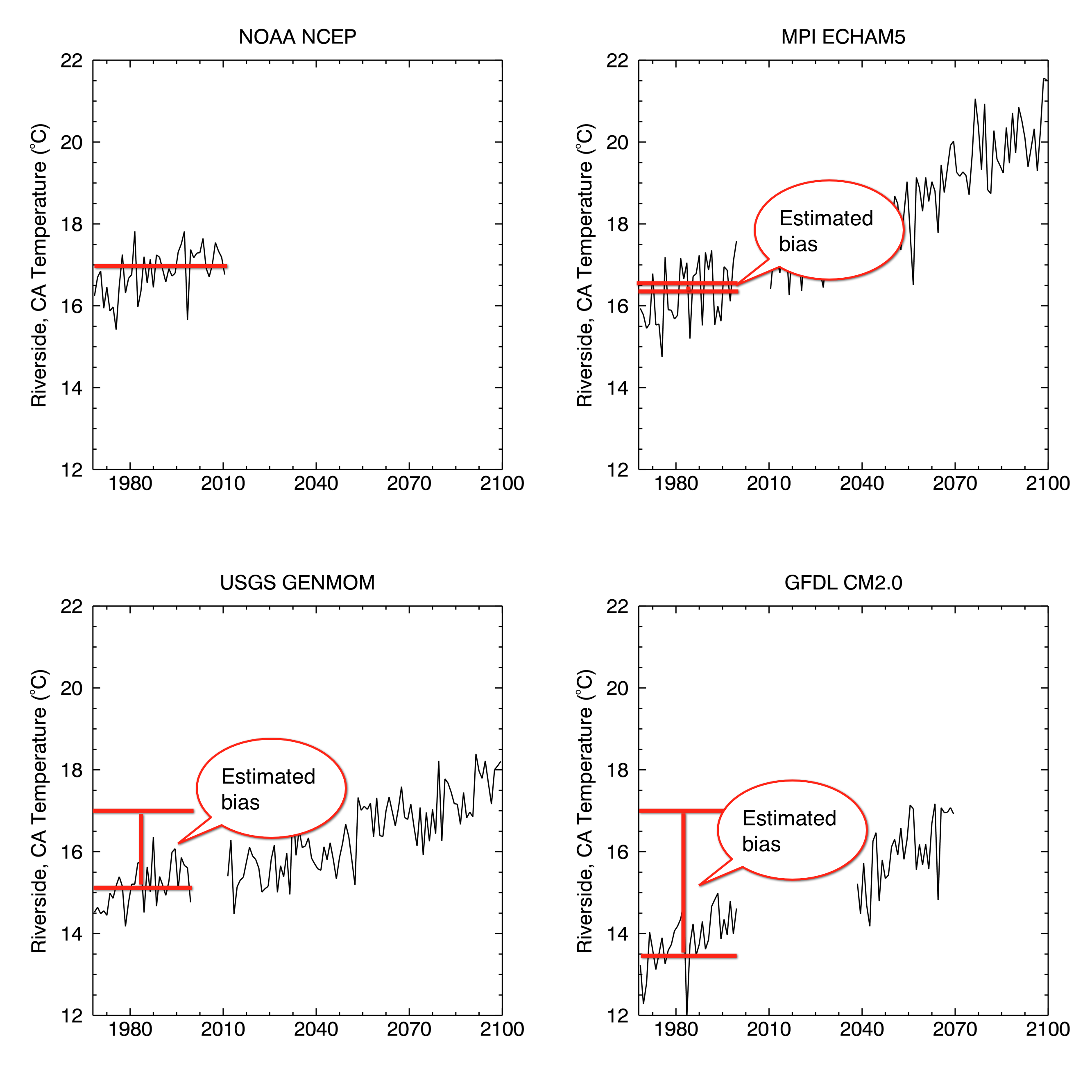
In the figure above from Climatology 401 we have estimated and highlighted the cold biases in the simulations. The horizontal red line at ~17ºC in all of the plots is the approximate the 1968-2010 average of the NOAA NCEP data. The 1968-1999 average for the ECHAM5 simulation is very close to that of the NOAA NCEP simulation, whereas USGS GENMOM is about 15ºC, and GFDL CM2.0 is about 13.5ºC. The difference between the NOAA NCEP 1980-1999 annual average temperature and the 1980-1999 annual average temperature of the other models can be used to apply a bias correction that effectively shifts the mean value of the biased time series to be the same as the NOAA NCEP mean. The following IDL code illustrates the process:
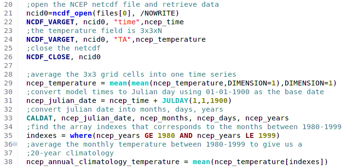
The first part of the IDL code (lines 1-19) defines directories, names the NetCDF files and opens the IDL graphics window is identical to the code we used in the Climatology 401 example and is not repeated here. The new additional code loads the temperature and dates for NOAA NCEP files (lines 21-26), averages the 9 grid cells into one value (line 29), and calculates the Julian and calendar dates (lines 31 and 33). The IDL “where” function is used to find the indices for the temperature array that are between 1980 and 1999 (line 35). Using the subset of the indices, we average the temperature of all the months between 1980 and 1999 to get the NOAA NCEP climatological mean temperature for Riverside, CA that will be used to correct the other models.
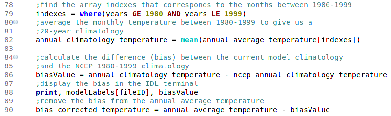
Similar to the above code, lines 79 and 82 calculate the annual climatological temperature for each model as the code is executed in the FOR loop. The model bias value is computed as the difference between the model climatology and the NOAA NCEP climatology (line 86). In this example, MPI ECHAM5 has a small bias of -0.3ºC, and USGS GENMOM and GFDL CM2.0 have biases of -1.5ºC and -2.8ºC, respectively (which are relatively small in magnitude for climate models). The calculated bias values are removed from each model temperature time series (line 90) and plotted in the graphics window. The code to plot the time series is the same as that used in Climatology 401.
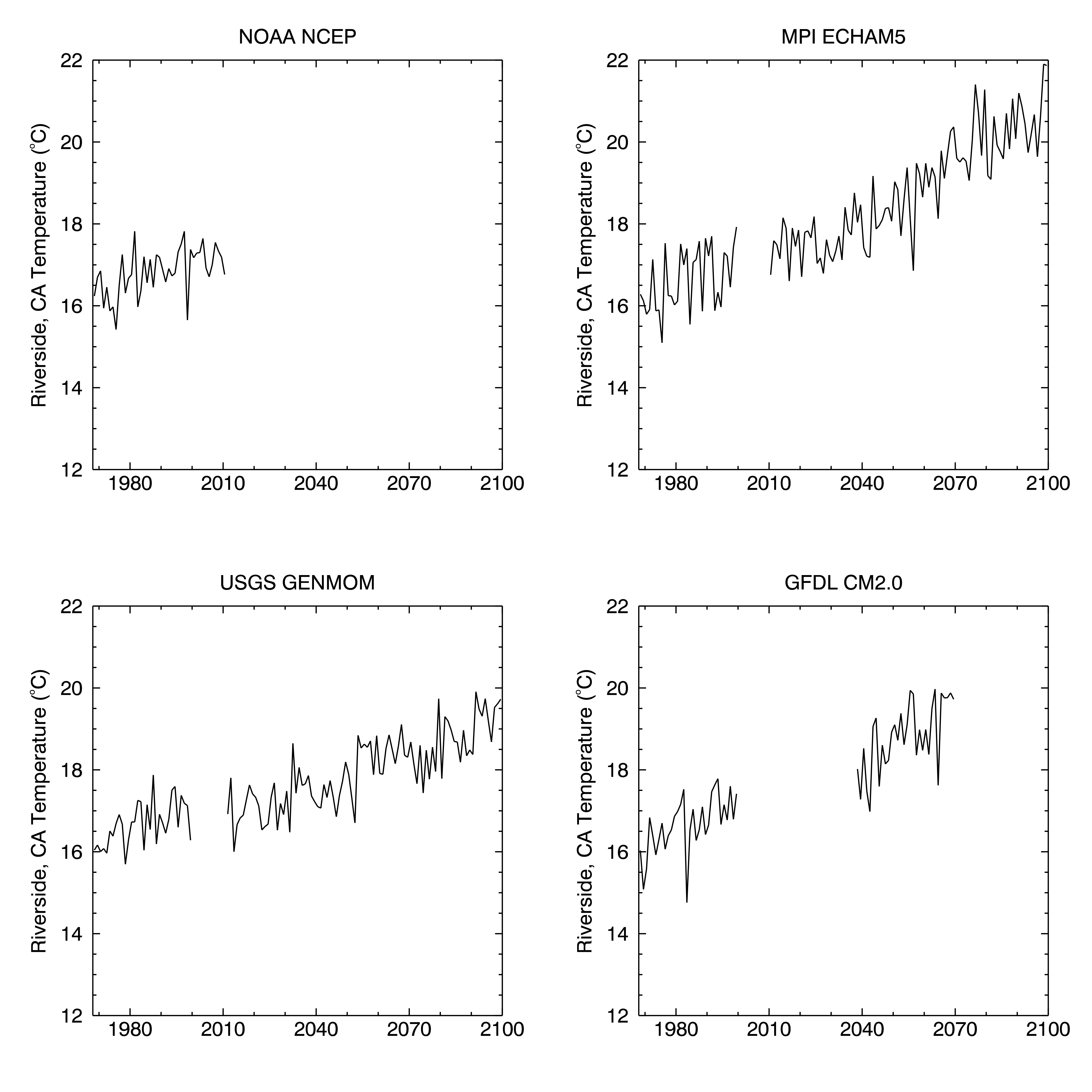
The result is a plot of the four, bias-corrected temperature time series for Riverside, CA. The average present-day values for the three models are now similar to the NOAA NCEP values and the future values are more comparable. All three models exhibit similar rates and magnitude and range of variability in the mid- to late 21st century.