Canadian National Fire DataBase (CNFDB)
1 (Canadian) National Fire DataBase
Canadian National Fire DataBase – http://cwfis.cfs.nrcan.gc.ca/datamart. The data come from the file NFDB_point_20141222.dbf (2014-12-22, accessed 2015-08-27), and are read directly using the read.dbf() function.
1.1 Overview
This is the Canadian National (Wildland) Fire Database. These data need some cleanup before analyis, in particular, the removal of points that plot over the ocean or the U.S. (including some points with 0.0 values for latitude and longtitude), and points with ambiguous dates “9980” or missing dates.
Read data directly from the distribution .dbf file, creating a data frame named cnfdb
library(foreign)
filename <- "e:/Projects/fire/CWFIS/distrib/NFDB_point_20141222.dbf"
cnfdb <- read.dbf(filename, as.is=TRUE)
List the first and last lines, total number of points, and structure of the data.
head(cnfdb); tail(cnfdb)## SRC_AGENCY FIRE_ID FIRENAME LATITUDE LONGITUDE YEAR MONTH DAY REP_DATE ATTK_DATE OUT_DATE DECADE
## 1 NL NA <NA> 47.73 -54.55 1955 6 22 1955-06-22 <NA> <NA> 1950-1959
## 2 NL NA <NA> 50.07 -56.12 1955 7 21 1955-07-21 <NA> <NA> 1950-1959
## 3 NL NA <NA> 48.09 -53.03 1956 5 13 1956-05-13 <NA> <NA> 1950-1959
## 4 NL NA <NA> 47.68 -53.83 1956 5 22 1956-05-22 <NA> <NA> 1950-1959
## 5 NL NA <NA> 47.00 -52.97 1956 6 3 1956-06-03 <NA> <NA> 1950-1959
## 6 NL NA <NA> 50.12 -56.13 1956 6 30 1956-06-30 <NA> <NA> 1950-1959
## SIZE_HA CAUSE PROTZONE FIRE_TYPE MORE_INFO CFS_REF_ID CFS_NOTE CFS_NOTE2 ACQ_DATE AG_SRCFILE
## 1 518 H NA <NA> <NA> NL-1955-NA <NA> <NA> 2008-07-24 <NA>
## 2 377 H NA <NA> <NA> NL-1955-NA <NA> <NA> 2008-07-24 <NA>
## 3 243 H NA <NA> <NA> NL-1956-NA <NA> <NA> 2008-07-24 <NA>
## 4 453 H NA <NA> <NA> NL-1956-NA <NA> <NA> 2008-07-24 <NA>
## 5 259 H NA <NA> <NA> NL-1956-NA <NA> <NA> 2008-07-24 <NA>
## 6 648 H NA <NA> <NA> NL-1956-NA <NA> <NA> 2008-07-24 <NA>## SRC_AGENCY FIRE_ID FIRENAME LATITUDE LONGITUDE YEAR MONTH
## 372095 PC-WLNP 2013WL1 Eskerine Complex Prescribed Fire Guard Burning 0.00000 0.0000 2013 2
## 372096 PC-WLNP 2013WL2 Eskerine Complex Guard Burning 49.12000 -113.8700 2013 4
## 372097 PC-WLNP 2013WL3 Blue Grouse Basin Prescribed Fire 49.12400 -114.1475 2013 9
## 372098 PC-WLNP 2013WL4 Eskerince Complex Guard Burning 49.11900 -113.8450 2013 11
## 372099 PC-WLNP 2013WL5 Eskerine Complex Guard Burning 49.12217 -113.8539 2013 11
## 372100 PC-YONP 2013YO1 Natural Bridge 51.38000 -116.5300 2013 7
## DAY REP_DATE ATTK_DATE OUT_DATE DECADE SIZE_HA CAUSE PROTZONE FIRE_TYPE
## 372095 28 2013-02-28 <NA> <NA> 2010-2019 3.0000 H-PB <NA> <NA>
## 372096 10 2013-04-10 <NA> <NA> 2010-2019 3.5000 H-PB <NA> <NA>
## 372097 15 2013-09-15 <NA> <NA> 2010-2019 4.0000 H-PB <NA> <NA>
## 372098 14 2013-11-14 <NA> <NA> 2010-2019 0.4000 H-PB <NA> <NA>
## 372099 27 2013-11-27 <NA> <NA> 2010-2019 0.9000 H-PB <NA> <NA>
## 372100 19 2013-07-19 <NA> <NA> 2010-2019 0.0012 H Full Response <NA>
## MORE_INFO CFS_REF_ID CFS_NOTE CFS_NOTE2 ACQ_DATE AG_SRCFILE
## 372095 Owner: Parks Canada PC-WLNP-2013-2013WL1 lat/long coords n/a <NA> 2014-01-31 <NA>
## 372096 Owner: Parks Canada PC-WLNP-2013-2013WL2 <NA> <NA> 2014-01-31 <NA>
## 372097 Owner: Parks Canada PC-WLNP-2013-2013WL3 <NA> <NA> 2014-01-31 <NA>
## 372098 Owner: Parks Canada PC-WLNP-2013-2013WL4 <NA> <NA> 2014-01-31 <NA>
## 372099 Owner: Parks Canada PC-WLNP-2013-2013WL5 <NA> <NA> 2014-01-31 <NA>
## 372100 Owner: Parks Canada PC-YONP-2013-2013YO1 <NA> <NA> 2014-01-31 <NA>str(cnfdb, strict.width="cut") # Variables in the data set## 'data.frame': 372100 obs. of 22 variables:
## $ SRC_AGENCY: chr "NL" "NL" "NL" "NL" ...
## $ FIRE_ID : chr "NA" "NA" "NA" "NA" ...
## $ FIRENAME : chr NA NA NA NA ...
## $ LATITUDE : num 47.7 50.1 48.1 47.7 47 ...
## $ LONGITUDE : num -54.5 -56.1 -53 -53.8 -53 ...
## $ YEAR : int 1955 1955 1956 1956 1956 1956 1956 1956 1957 1957 ...
## $ MONTH : int 6 7 5 5 6 6 7 7 5 5 ...
## $ DAY : int 22 21 13 22 3 30 12 27 13 17 ...
## $ REP_DATE : Date, format: "1955-06-22" "1955-07-21" "1956-05-13" ...
## $ ATTK_DATE : Date, format: NA NA NA ...
## $ OUT_DATE : Date, format: NA NA NA ...
## $ DECADE : chr "1950-1959" "1950-1959" "1950-1959" "1950-1959" ...
## $ SIZE_HA : num 518 377 243 453 259 648 202 688 243 243 ...
## $ CAUSE : chr "H" "H" "H" "H" ...
## $ PROTZONE : chr "NA" "NA" "NA" "NA" ...
## $ FIRE_TYPE : chr NA NA NA NA ...
## $ MORE_INFO : chr NA NA NA NA ...
## $ CFS_REF_ID: chr "NL-1955-NA" "NL-1955-NA" "NL-1956-NA" "NL-1956-NA" ...
## $ CFS_NOTE : chr NA NA NA NA ...
## $ CFS_NOTE2 : chr NA NA NA NA ...
## $ ACQ_DATE : Date, format: "2008-07-24" "2008-07-24" "2008-07-24" ...
## $ AG_SRCFILE: chr NA NA NA NA ...
## - attr(*, "data_types")= chr "C" "C" "C" "N" ...1.2 Clean up
Clean up was done in several steps, first flagging the points located over the ocean, or outside of Canada, and then flagging other invalid points. After invalid points are flagged, they are removed from the data.
1.2.1 Points outside of Canada
First, get the Natural Earth administrative outlines to use as a basemap and for trimming the data set to include only those points in Canada. These are available at http://www.naturalearthdata.com/downloads/.
Read polygon outline files for Canada and the U.S. Load various packages first.
library(sp)
library(maptools)
## Checking rgeos availability: TRUElibrary(rgdal)## rgdal: version: 1.2-7, (SVN revision 660)
## Geospatial Data Abstraction Library extensions to R successfully loaded
## Loaded GDAL runtime: GDAL 2.0.1, released 2015/09/15
## Path to GDAL shared files: C:/Users/bartlein/Documents/R/win-library/3.4/rgdal/gdal
## Loaded PROJ.4 runtime: Rel. 4.9.2, 08 September 2015, [PJ_VERSION: 492]
## Path to PROJ.4 shared files: C:/Users/bartlein/Documents/R/win-library/3.4/rgdal/proj
## Linking to sp version: 1.2-4library(rgeos)## rgeos version: 0.3-23, (SVN revision 546)
## GEOS runtime version: 3.5.0-CAPI-1.9.0 r4084
## Linking to sp version: 1.2-4
## Polygon checking: TRUERead the “administrative” (country outlines) shapefile.
admin_shapefile <- "e:/DataVis/RMaps/mapfiles/ne_10m_admin_0_countries/ne_10m_admin_0_countries.shp"
layer <- ogrListLayers(admin_shapefile)
# summarize contents of admin_shapefile
#ogrInfo(admin_shapefile, layer=layer)
# read the shapefile
admin_poly_shp <- readOGR(admin_shapefile, layer=layer)
## OGR data source with driver: ESRI Shapefile
## Source: "e:/DataVis/RMaps/mapfiles/ne_10m_admin_0_countries/ne_10m_admin_0_countries.shp", layer: "ne_10m_admin_0_countries"
## with 255 features
## It has 65 fields# summarize and plot the whole shapefile
#summary(admin_poly_shp)
#plot(admin_poly_shp, bor="gray")
# get the country codes
#admin_poly_shp$adminGet the Canada and U.S. outlines
# Canada is 40, U.S. is 239
# get Canada and U.S. outlines
can_poly_shp <- admin_poly_shp[40,]
us_poly_shp <- admin_poly_shp[239,]
Map the data. This particular map scope does not include the stack of points that plot at 0N, 0E (i.e. those with LATITUDE and LONGITUDE equal to zero)
plot(cnfdb$LATITUDE ~ cnfdb$LONGITUDE, ylim=c(40,85), xlim=c(-145,-50), type="n",
  xlab="Longitude", ylab="Latitude")
points(cnfdb$LATITUDE ~ cnfdb$LONGITUDE, pch=16, cex=0.3, col="red")
plot(us_poly_shp, bor="lightblue", add=TRUE)
plot(can_poly_shp, bor="black", add=TRUE)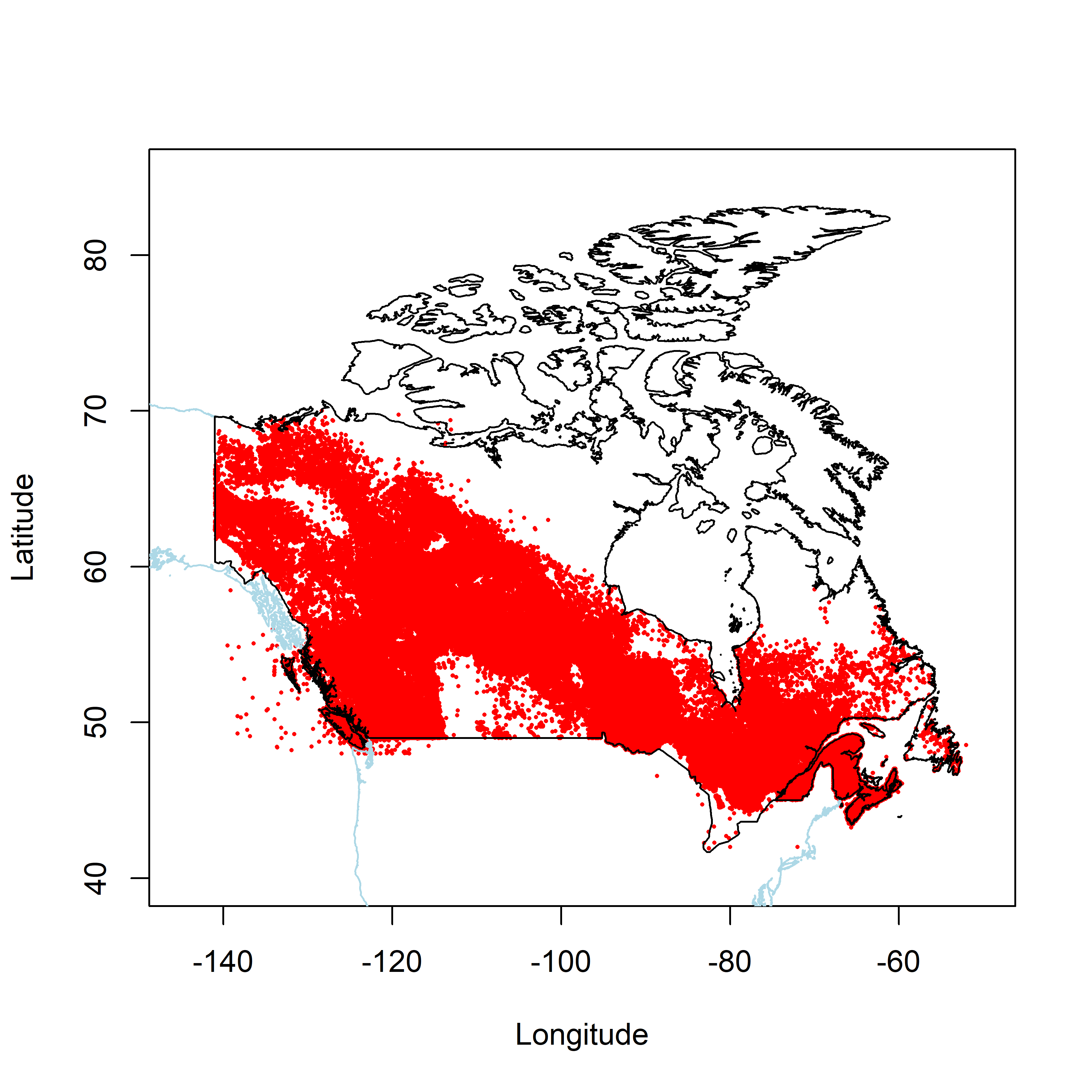
There are a number of points that plot in the ocean, or in the U.S. The particular problem in western Canada can be seen by zooming into the Pacific Northwest:
plot(cnfdb$LATITUDE ~ cnfdb$LONGITUDE, ylim=c(48,60), xlim=c(-140,-115), type="n",
  xlab="Longitude", ylab="Latitude")
points(cnfdb$LATITUDE ~ cnfdb$LONGITUDE, pch=16, cex=0.3, col="red")
plot(us_poly_shp, bor="lightblue", add=TRUE)
plot(can_poly_shp, bor="black", add=TRUE)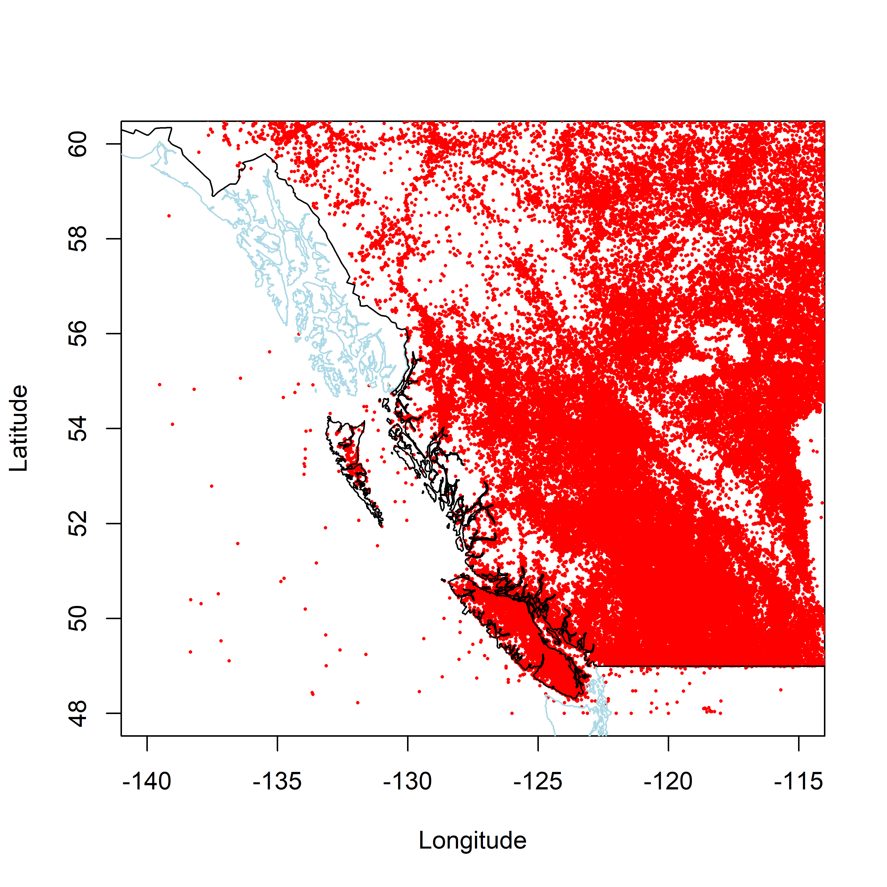
Next, add a couple of variables cnfdb$seqnum and cnfdb$valid_point for keeping track of original observation order and points that are identified as invalid.
cnfdb$seqnum <- seq(1:length(cnfdb[,1]))
cnfdb$validpts <- rep(1,length(cnfdb[,1]))
Make a spatial points data frame to trim on the Canada outline in order to identify out-of-bounds points.
unproj_projstr <- proj4string(can_poly_shp)
can_df <- data.frame(cbind(cnfdb$LONGITUDE,cnfdb$LATITUDE))
can_pts <- SpatialPointsDataFrame(coords=data.frame(cbind(cnfdb$LONGITUDE,cnfdb$LATITUDE)),
  data=data.frame(cnfdb$seqnum), coords.nrs=c(1,2), proj4string=CRS(unproj_projstr))
#summary(can_pts)
#points(can_pts, pch=16, col="gray50", cex=0.01)
Trim the points using the Canada outline.
ptm <- proc.time() # timer
can_pts_valid <- gIntersects(can_poly_shp, can_pts, byid=TRUE)
proc.time() - ptm # how long?
## user system elapsed
## 1.30 0.05 1.34length(can_pts_valid)## [1] 372100table(can_pts_valid)## can_pts_valid
## FALSE TRUE
## 4217 367883So there are 4217 that plot outside of Canada. Set the valid points flag to 0 for those points. Plot all points in red and overlay the valid points (so far), in blue.
cnfdb$validpts[can_pts_valid == FALSE] <- 0
plot(cnfdb$LATITUDE ~ cnfdb$LONGITUDE, ylim=c(40,85), xlim=c(-145,-50), type="n",
  xlab="Longitude", ylab="Latitude")
plot(us_poly_shp, bor="lightblue", add=TRUE)
plot(can_poly_shp, bor="black", add=TRUE)
points(cnfdb$LATITUDE ~ cnfdb$LONGITUDE, pch=16, cex=0.2, col="red")
points(cnfdb$LATITUDE[cnfdb$validpts == 1] ~ cnfdb$LONGITUDE[cnfdb$validpts == 1],
  pch=16, col="blue", cex=0.2)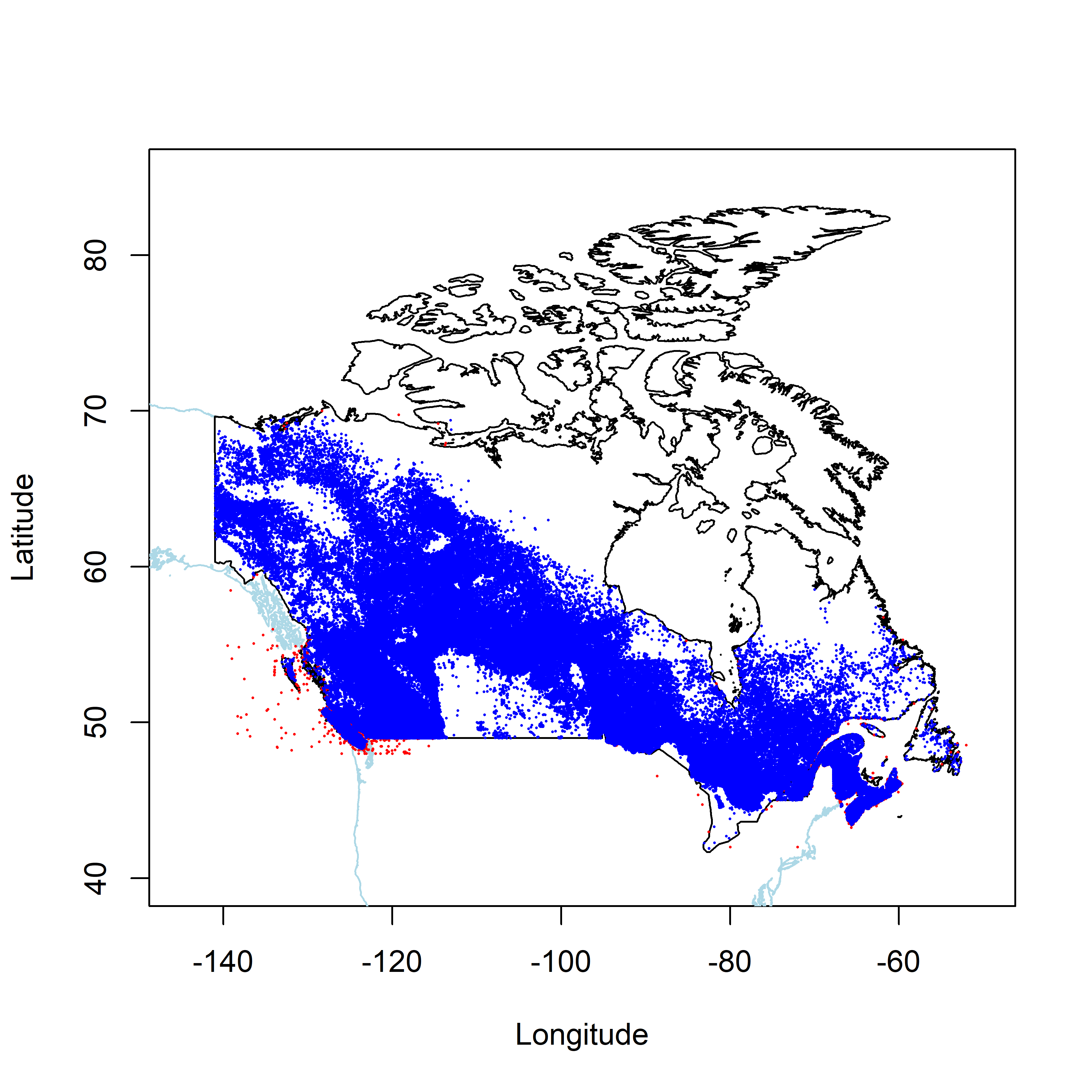
1.2.2 Other points
Next, discover points that have out-of-range YEAR values:
The points with YEAR values outside the range 1980 through 2014 can be flagged as follows.
cnfdb$validpts[cnfdb$YEAR < 1980] <- 0
cnfdb$validpts[cnfdb$YEAR > 2014] <- 0
table(cnfdb$validpts)
##
## 0 1
## 90993 281107Set flags for MONTH and DAY values that are missing or 0, or out of bounds.
cnfdb$MONTH[cnfdb$MONTH == 0] <- NA
cnfdb$DAY[cnfdb$DAY == 0] <- NA
cnfdb$DAY[cnfdb$DAY > 31] <- NA
cnfdb$validpt[is.na(cnfdb$MONTH) == TRUE] <- 0
cnfdb$validpt[is.na(cnfdb$DAY) == TRUE] <- 0
table(cnfdb$validpt)
##
## 0 1
## 94872 277228There is one fire with SIZE_HA equal to -1.0. Set SIZE_HA to 0.0.
cnfdb[which.min(cnfdb$SIZE_HA),]## SRC_AGENCY FIRE_ID FIRENAME LATITUDE LONGITUDE YEAR MONTH DAY REP_DATE ATTK_DATE
## 36019 MB EA-512-050-97 <NA> 51.517 -95.1 1997 6 12 1997-06-12 1997-06-12
## OUT_DATE DECADE SIZE_HA CAUSE PROTZONE FIRE_TYPE MORE_INFO CFS_REF_ID CFS_NOTE
## 36019 1997-06-13 1990-1999 -1 L NA <NA> <NA> MB-1997-EA-512-050-97 <NA>
## CFS_NOTE2 ACQ_DATE AG_SRCFILE seqnum validpts validpt
## 36019 <NA> 2008-07-24 <NA> 36019 1 1cnfdb[which.min(cnfdb$SIZE_HA),]$SIZE_HA <- 0.0There are now 277228 valid points. Commit the changes.
cnfdb <- cnfdb[cnfdb$validpt == 1,]
length(cnfdb[,1])
## [1] 277228summary(cnfdb)## SRC_AGENCY FIRE_ID FIRENAME LATITUDE LONGITUDE
## Length:277228 Length:277228 Length:277228 Min. :41.92 Min. :-141.00
## Class :character Class :character Class :character 1st Qu.:49.23 1st Qu.:-120.19
## Mode :character Mode :character Mode :character Median :51.02 Median :-114.61
## Mean :51.95 Mean :-105.15
## 3rd Qu.:54.74 3rd Qu.: -90.66
## Max. :69.60 Max. : -52.69
##
## YEAR MONTH DAY REP_DATE ATTK_DATE
## Min. :1980 Min. : 1.000 Min. : 1.00 Min. :1955-05-19 Min. :1899-12-30
## 1st Qu.:1989 1st Qu.: 6.000 1st Qu.: 8.00 1st Qu.:1989-04-29 1st Qu.:1986-06-09
## Median :1997 Median : 7.000 Median :16.00 Median :1997-05-15 Median :1990-06-23
## Mean :1997 Mean : 6.688 Mean :15.62 Mean :1997-04-28 Mean :1990-04-18
## 3rd Qu.:2006 3rd Qu.: 8.000 3rd Qu.:23.00 3rd Qu.:2006-06-01 3rd Qu.:1995-06-30
## Max. :2014 Max. :12.000 Max. :31.00 Max. :2014-04-28 Max. :2207-08-30
## NA's :203467
## OUT_DATE DECADE SIZE_HA CAUSE PROTZONE
## Min. :1980-04-02 Length:277228 Min. : 0.0 Length:277228 Length:277228
## 1st Qu.:1988-06-14 Class :character 1st Qu.: 0.0 Class :character Class :character
## Median :1993-07-10 Mode :character Median : 0.1 Mode :character Mode :character
## Mean :1995-03-15 Mean : 296.1
## 3rd Qu.:2001-07-10 3rd Qu.: 1.0
## Max. :2013-11-13 Max. :624883.0
## NA's :152997
## FIRE_TYPE MORE_INFO CFS_REF_ID CFS_NOTE CFS_NOTE2
## Length:277228 Length:277228 Length:277228 Length:277228 Length:277228
## Class :character Class :character Class :character Class :character Class :character
## Mode :character Mode :character Mode :character Mode :character Mode :character
##
##
##
##
## ACQ_DATE AG_SRCFILE seqnum validpts validpt
## Min. :1899-12-30 Length:277228 Min. : 25 Min. :1 Min. :1
## 1st Qu.:2010-11-09 Class :character 1st Qu.: 87874 1st Qu.:1 1st Qu.:1
## Median :2012-08-30 Mode :character Median :160590 Median :1 Median :1
## Mean :2011-09-23 Mean :186710 Mean :1 Mean :1
## 3rd Qu.:2012-08-30 3rd Qu.:298564 3rd Qu.:1 3rd Qu.:1
## Max. :2014-06-17 Max. :372100 Max. :1 Max. :1
## NA's :77660Save the cleaned up data
outworkspace="cnfdb_cleaned.RData"
save.image(file=outworkspace)
Total number of valid points:
length(cnfdb[,1])## [1] 277228Map the points.
plot(cnfdb$LATITUDE ~ cnfdb$LONGITUDE, ylim=c(40,85), xlim=c(-145,-50), type="n",
  xlab="Longitude", ylab="Latitude")
points(cnfdb$LATITUDE ~ cnfdb$LONGITUDE, pch=16, cex=0.3, col="red")
plot(us_poly_shp, bor="lightblue", add=TRUE)
plot(can_poly_shp, bor="black", add=TRUE)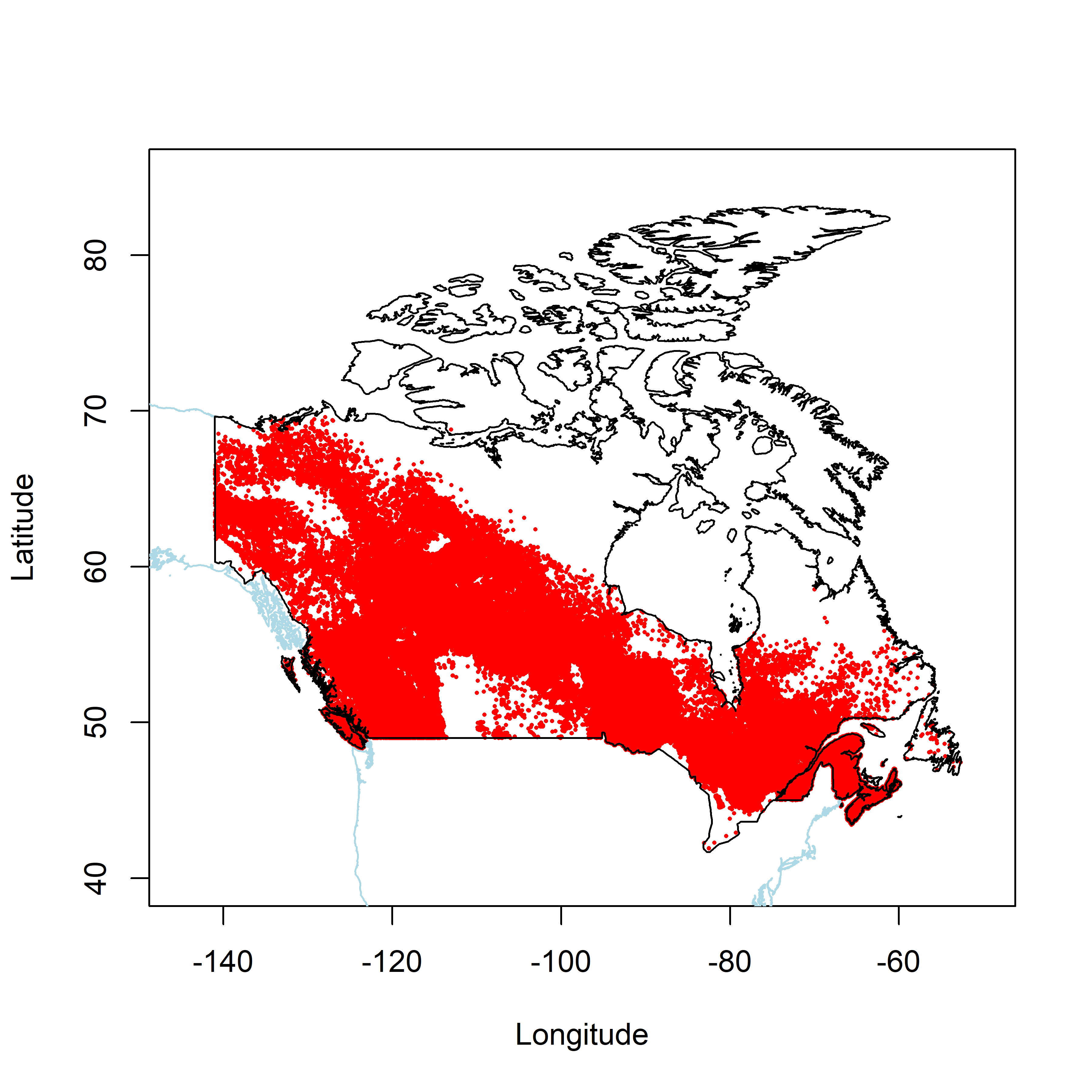
1.3 Analysis of the Canadian data
Number of fires by different causes:
# H, human; H-PB, prescribed burn; L, Lightning; Re, ??; U, unknown
table(cnfdb$CAUSE)
##
## H H-PB L Re U
## 144462 101 119272 86 12369Number of fires by agency:
table(cnfdb$SRC_AGENCY)##
## AB BC MB NB NL NS NWT ON PC-BA PC-BANP PC-BP PC-BT PC-CB
## 40439 100690 15268 8767 348 8155 9166 47957 136 3 4 4 3
## PC-EI PC-FO PC-FW PC-GB PC-GF PC-GI PC-GL PC-GLNP PC-GR PC-GRNP PC-JA PC-JANP PC-KE
## 27 1 1 1 61 1 45 4 80 3 143 3 6
## PC-KG PC-KL PC-KO PC-KONP PC-LM PC-NA PC-NANP PC-PA PC-PANP PC-PE PC-PP PC-PPNP PC-PU
## 25 2 86 5 26 16 9 66 5 1 2 1 51
## PC-RE PC-RENP PC-RM PC-RMNP PC-SL PC-TN PC-VU PC-WAFU PC-WB PC-WBNP PC-WL PC-WLNP PC-YO
## 21 2 47 2 5 2 1 2 1050 50 24 4 43
## PC-YONP QC SK YT
## 1 18218 21454 4691Recode multiple “PC” agencies:
cnfdb$agency <- cnfdb$SRC_AGENCY
cnfdb$agency[substr(cnfdb$agency,1,2)=="PC"]  <- "PC"
table(cnfdb$agency)
##
## AB BC MB NB NL NS NWT ON PC QC SK YT
## 40439 100690 15268 8767 348 8155 9166 47957 2075 18218 21454 4691Total number of fires each year:
hist(cnfdb$YEAR, xlim=c(1980,2015), ylim=c(0,20000),breaks=seq(1979.5,2014.5,by=1),
  main="cnfdb, All Fires, All Agencies")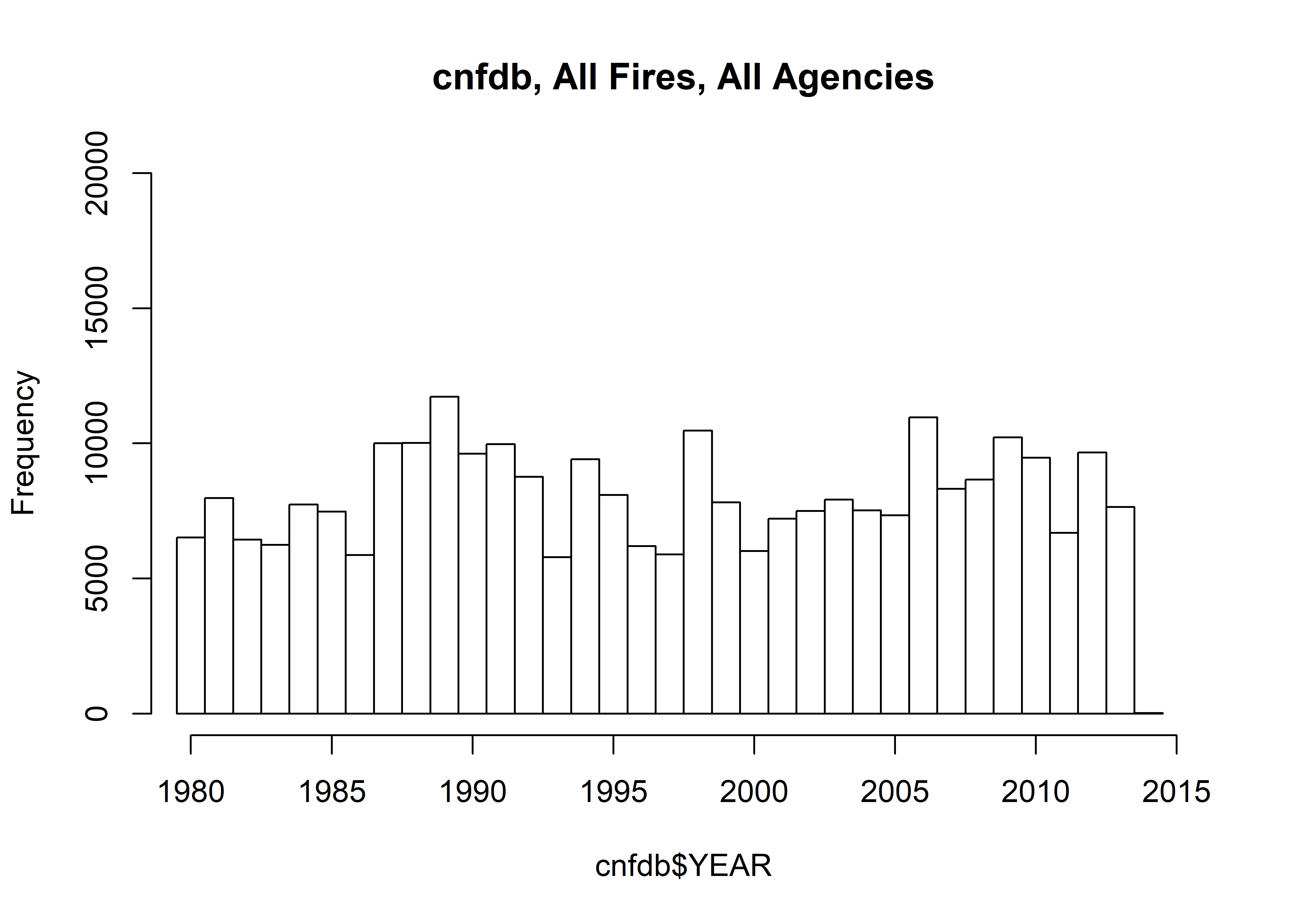
table(cnfdb$YEAR)##
## 1980 1981 1982 1983 1984 1985 1986 1987 1988 1989 1990 1991 1992 1993 1994 1995 1996
## 6522 7982 6435 6249 7734 7472 5868 10005 10013 11729 9615 9969 8766 5796 9414 8096 6197
## 1997 1998 1999 2000 2001 2002 2003 2004 2005 2006 2007 2008 2009 2010 2011 2012 2013
## 5895 10469 7822 6015 7216 7503 7923 7520 7335 10968 8322 8661 10224 9466 6694 9663 7649
## 2014
## 211.3.1 Time series
Plot the total area burned each year.
total_by_year <- tapply(cnfdb$SIZE_HA, cnfdb$YEAR, sum)
total_by_year
## 1980 1981 1982 1983 1984 1985 1986 1987 1988
## 4820920.89 6235378.68 1737789.11 2012224.08 755999.24 958098.31 1108525.09 1049219.86 1351563.91
## 1989 1990 1991 1992 1993 1994 1995 1996 1997
## 7683371.32 933090.60 1617000.05 854200.94 1971161.14 6262408.68 6275029.11 1930011.86 560026.41
## 1998 1999 2000 2001 2002 2003 2004 2005 2006
## 4663267.26 1741915.51 418722.94 565241.42 2675994.49 1199920.66 3182395.04 1703130.85 2084627.91
## 2007 2008 2009 2010 2011 2012 2013 2014
## 1767367.36 1645102.69 708449.37 3016437.55 2399845.71 1784314.67 4415786.58 13.76year <- as.numeric(unlist(dimnames(total_by_year)))
total_by_year <- as.numeric(total_by_year)
plot(total_by_year ~ year, pch=16, type="o", lwd=3, col="red", main="Total Area Burned (ha) (Canada)")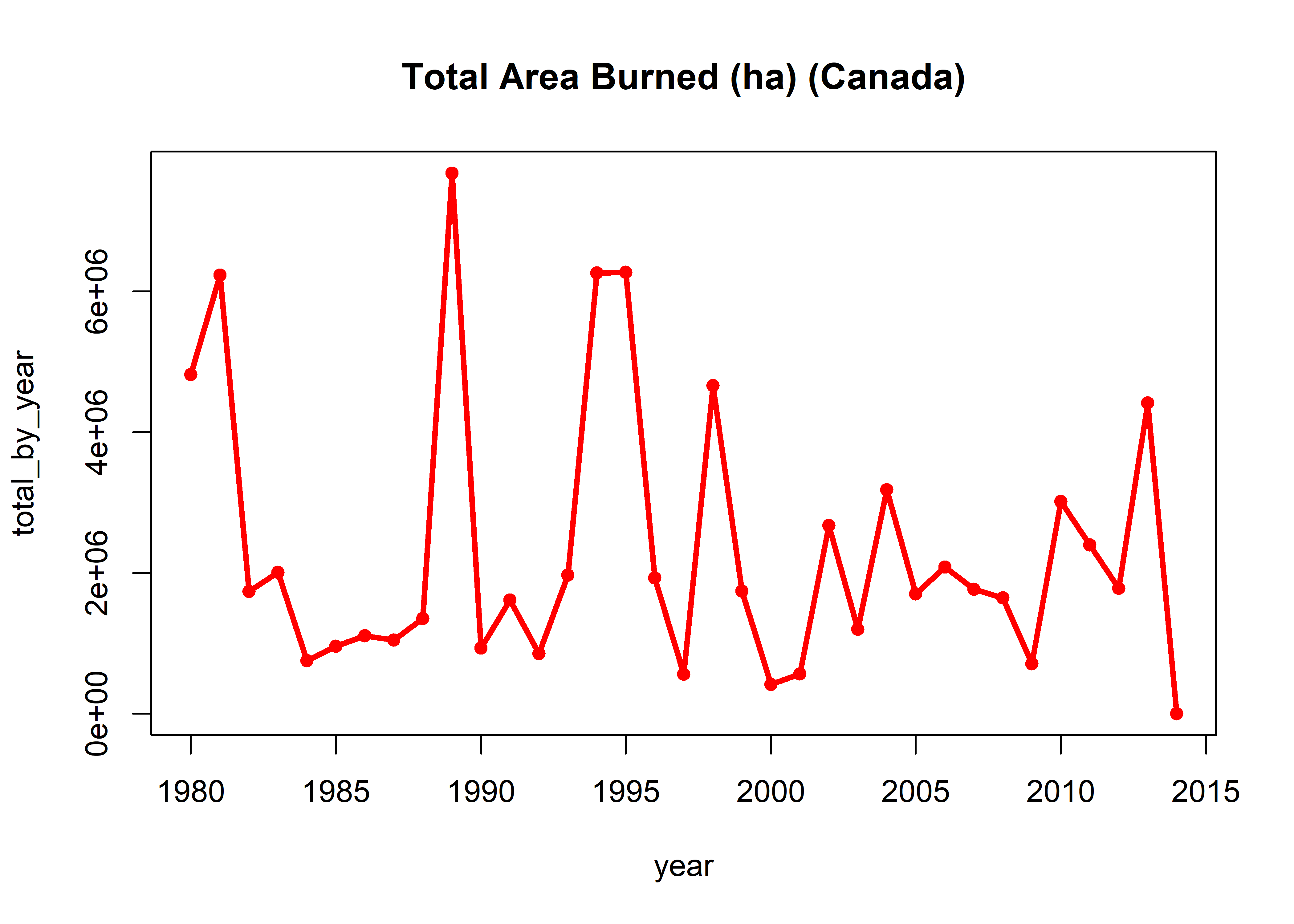
Mean area burned by year:
mean_by_year <- tapply(cnfdb$SIZE_HA, cnfdb$YEAR, mean)
mean_by_year
## 1980 1981 1982 1983 1984 1985 1986 1987
## 739.1783027 781.1799897 270.0526977 322.0073740 97.7500957 128.2251480 188.9102062 104.8695512
## 1988 1989 1990 1991 1992 1993 1994 1995
## 134.9809158 655.0747140 97.0453042 162.2028338 97.4447798 340.0899137 665.2229318 775.0777063
## 1996 1997 1998 1999 2000 2001 2002 2003
## 311.4429337 95.0002392 445.4357873 222.6943883 69.6131235 78.3316818 356.6566027 151.4477676
## 2004 2005 2006 2007 2008 2009 2010 2011
## 423.1908302 232.1923456 190.0645434 212.3729101 189.9437349 69.2927783 318.6602101 358.5069777
## 2012 2013 2014
## 184.6543174 577.3024679 0.6552381year <- as.numeric(unlist(dimnames(mean_by_year)))
mean_by_year <- as.numeric(mean_by_year)
plot(mean_by_year ~ year, pch=16, type="o", lwd=3, col="red", main="Mean Area Burned (ha) (Canada)")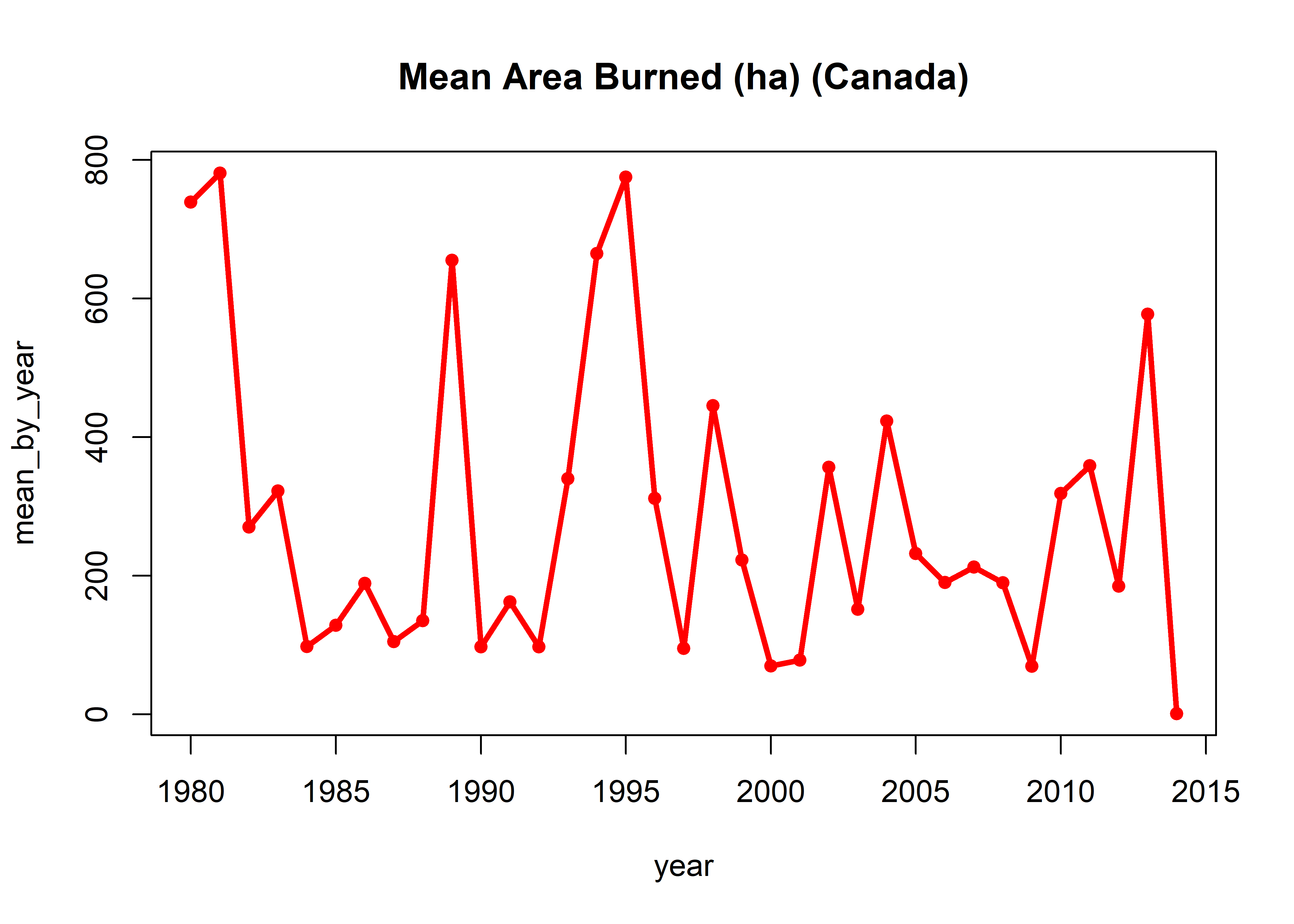
Number of fires by different causes:
# H=human, H-PB=prescribed burn, L=lighting, Re=???, U=unknown
table(cnfdb$CAUSE)
##
## H H-PB L Re U
## 144462 101 119272 86 123691.3.2 Start-day histograms
Get start-day numbers (i.e. day in year):
library(lubridate)##
## Attaching package: 'lubridate'## The following object is masked from 'package:base':
##
## datecnfdb$startdaynum <- yday((strptime(cnfdb$REP_DATE, "%Y-%m-%d")))
cnfdb$startday <- cnfdb$DAY
cnfdb$startmon <- cnfdb$MONTHHistograms of start-day number (day in year startdaynum) for all data, human and lightning:
hist(cnfdb$startdaynum, breaks=seq(-0.5,366.5,by=1), freq=-TRUE,
  ylim=c(0,5000), xlim=c(0,400), main="startdaynum (All Fires)")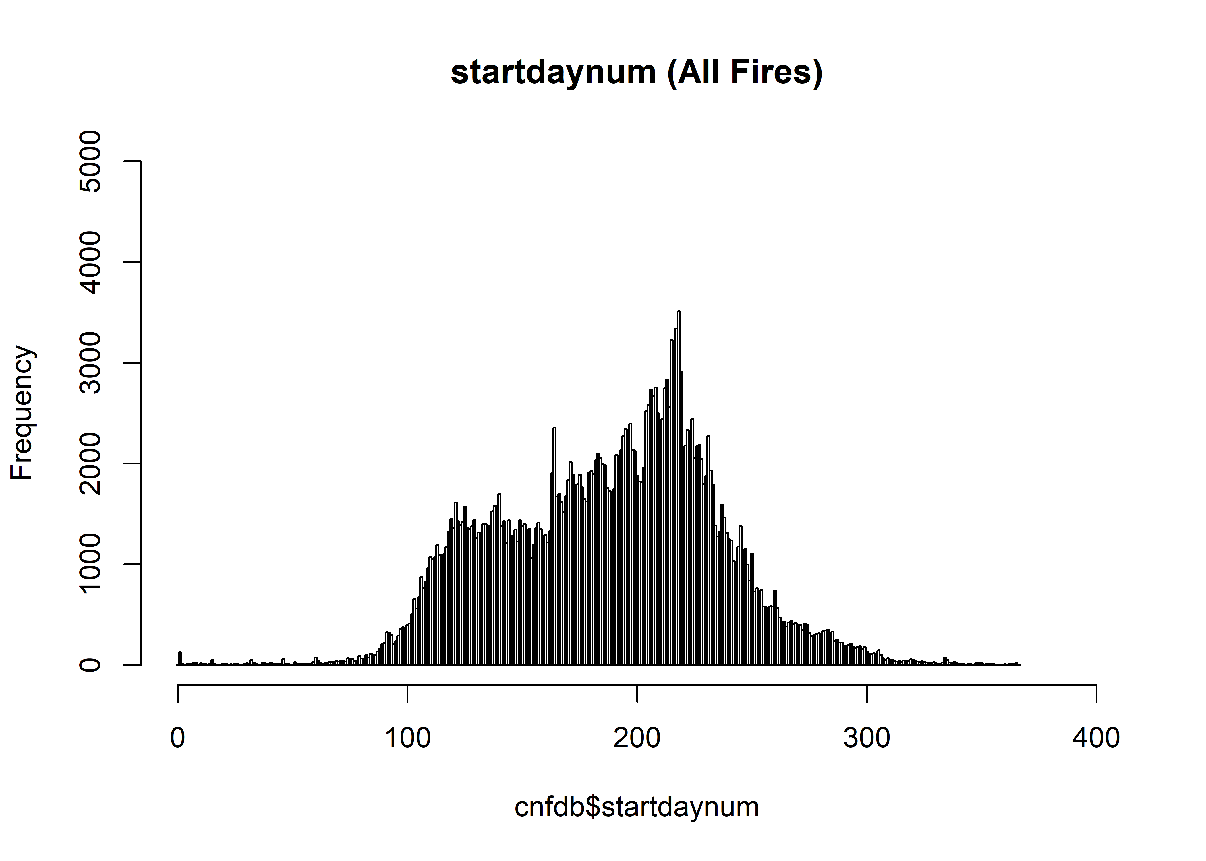
hist(cnfdb$startdaynum[cnfdb$CAUSE=="H"], breaks=seq(-0.5,366.5,by=1), freq=-TRUE,
  xlim=c(0,400), ylim=c(0,5000), main="startdaynum (Human)")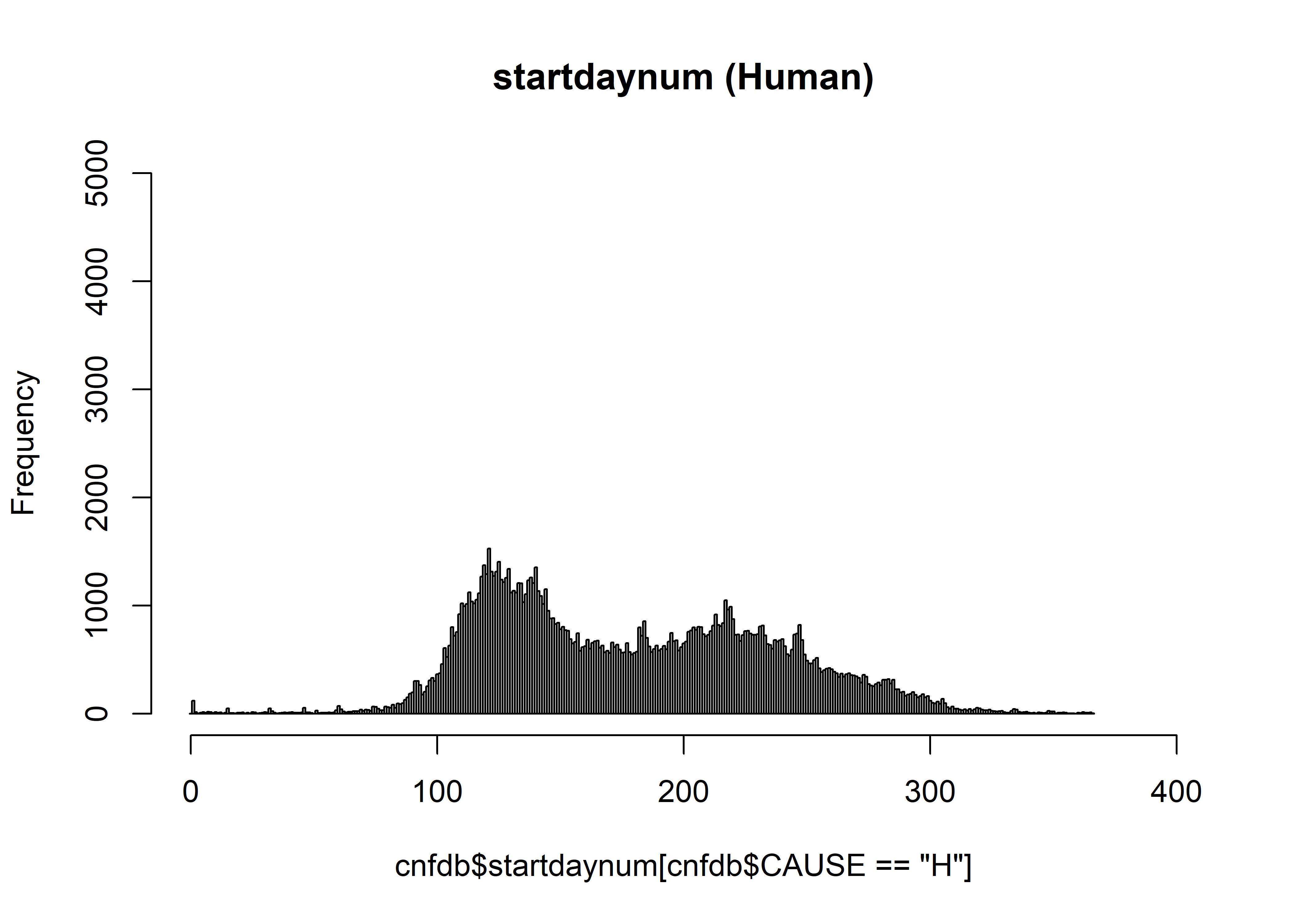
hist(cnfdb$startdaynum[cnfdb$CAUSE=="L"], breaks=seq(-0.5,366.5,by=1), freq=-TRUE,
  xlim=c(0,400), ylim=c(0,5000), main="startdaynum (Lightning)")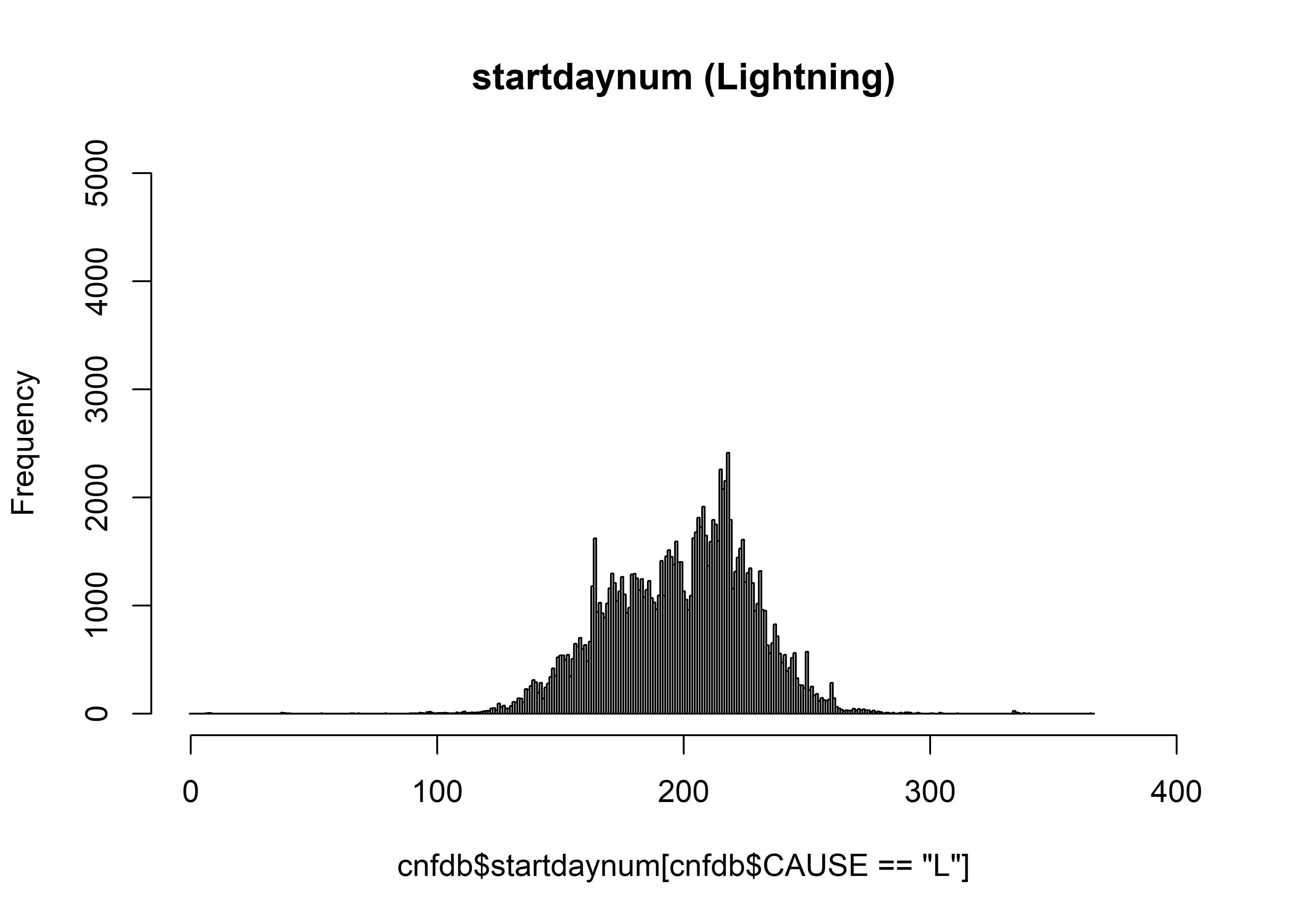
Histograms of the start day (in each month) over all months and years:
hist(cnfdb$startday, breaks=seq(-0.5,31.5,by=1), freq=-TRUE, ylim=c(0,30000),
  main="Start day of month (All Fires)")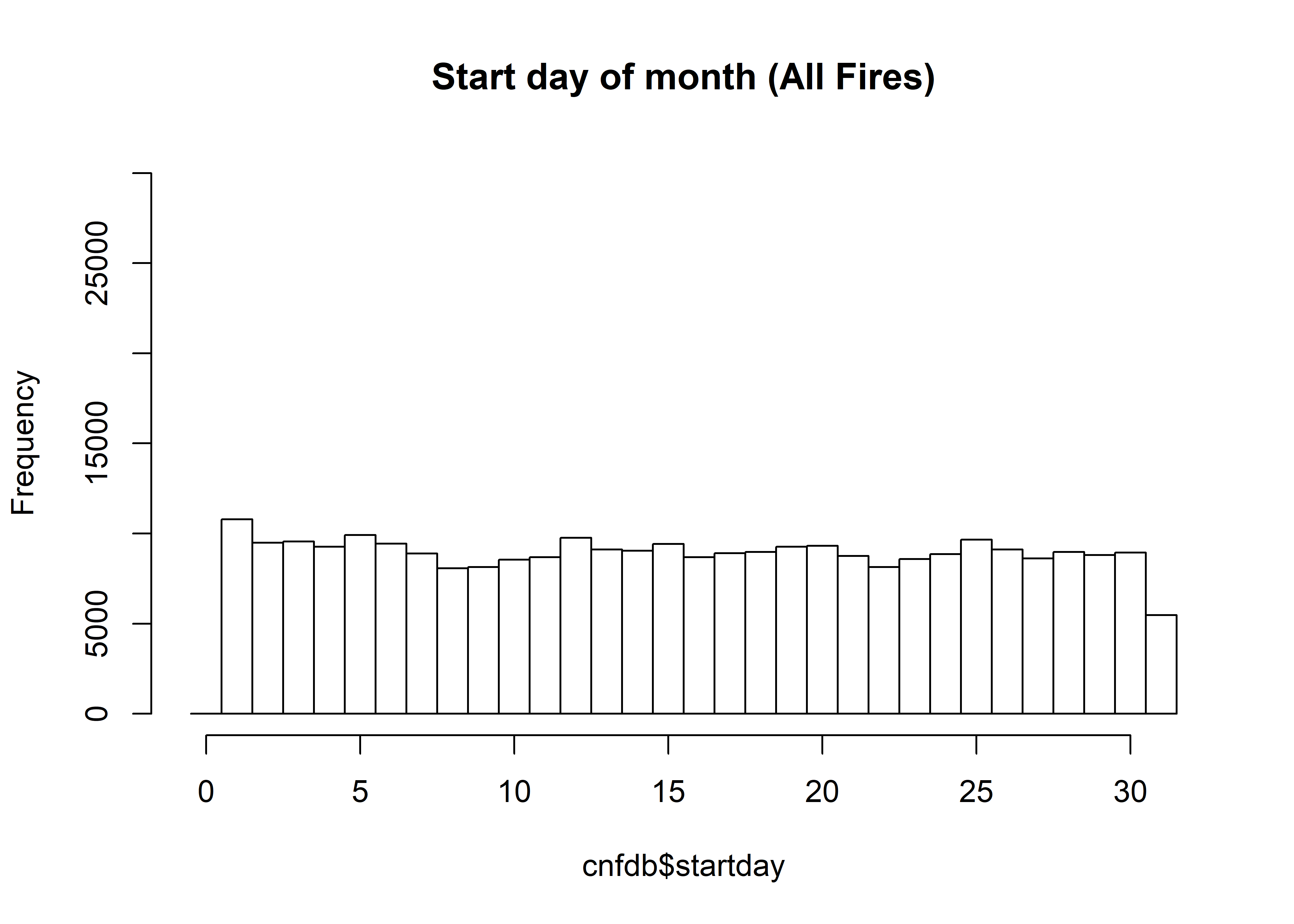
hist(cnfdb$startday[cnfdb$CAUSE=="H"], breaks=seq(-0.5,31.5,by=1),
  freq=-TRUE, ylim=c(0,30000), main="Start day of month (Human Fires)")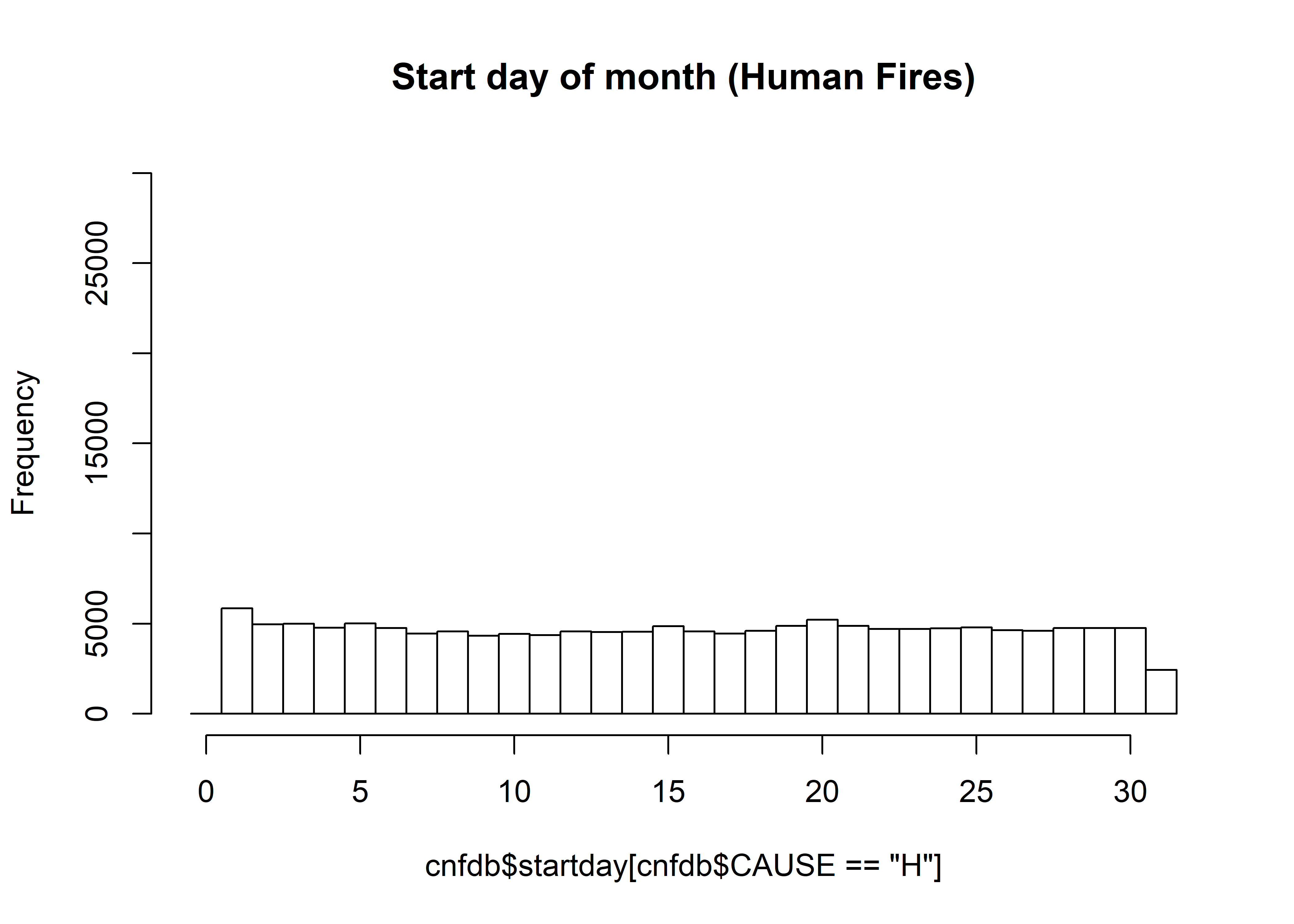
hist(cnfdb$startday[cnfdb$CAUSE=="L"], breaks=seq(-0.5,31.5,by=1),
  freq=-TRUE, ylim=c(0,30000), main="Start day of month (Lightning Fires)")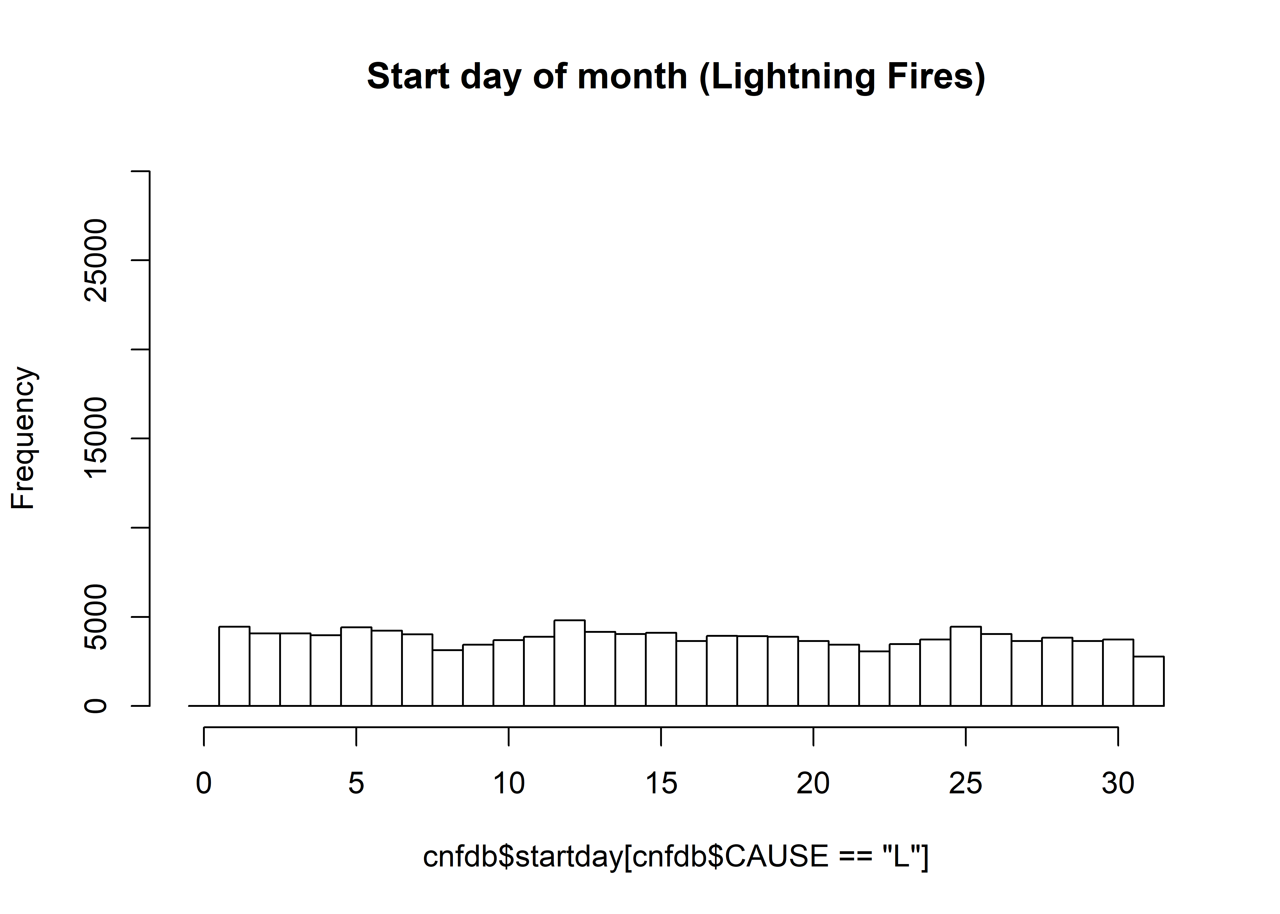
Histograms of log10 fire sizes (note the small values added to avoid 0’s):
hist(log10(cnfdb$SIZE_HA+0.0001), xlim=c(-6,8), breaks=20,
  main="All Fires")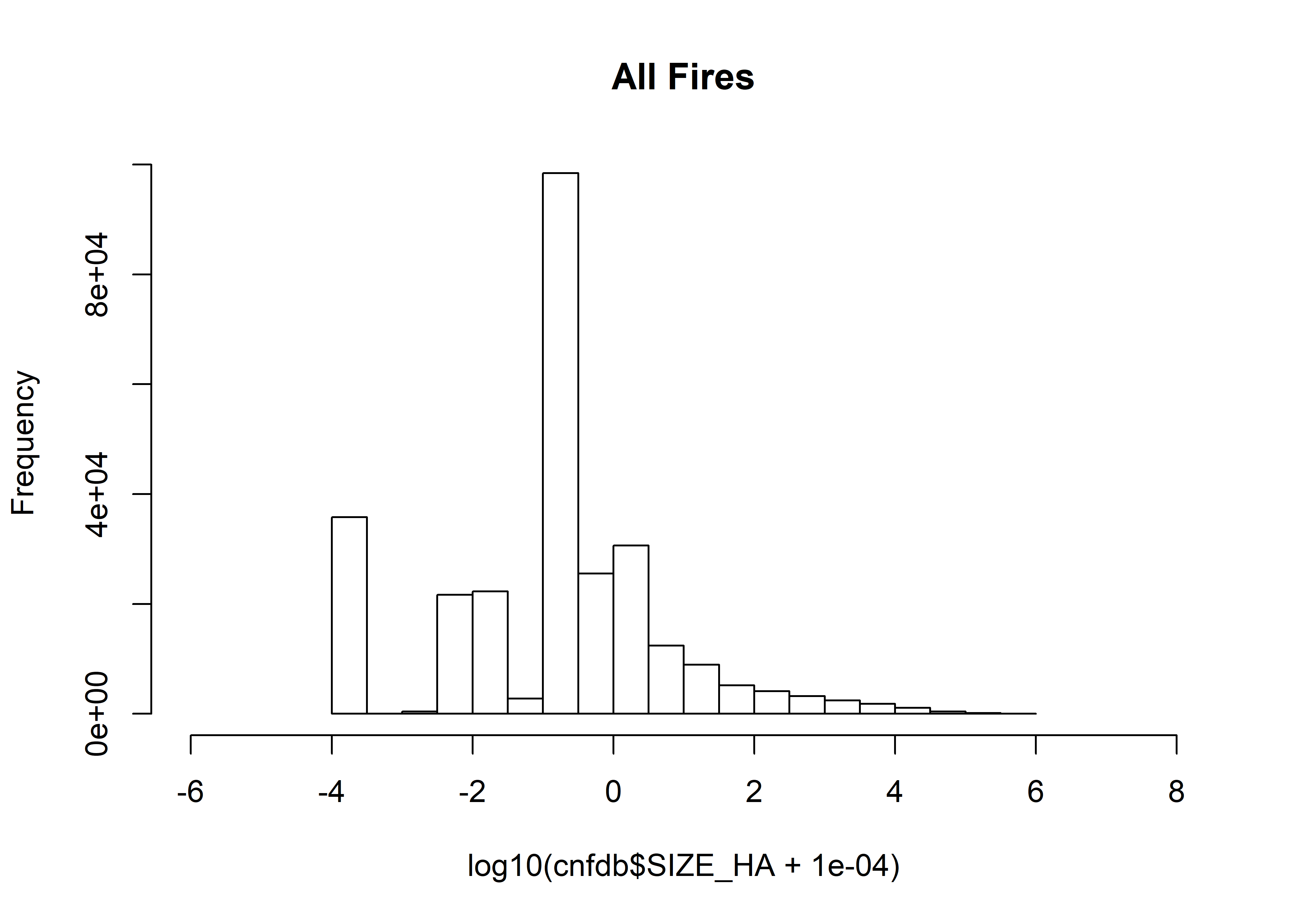
hist(log10(cnfdb$SIZE_HA[cnfdb$CAUSE == "H"]+0.0001), xlim=c(-6,8), breaks=20,
  main="Human Fires")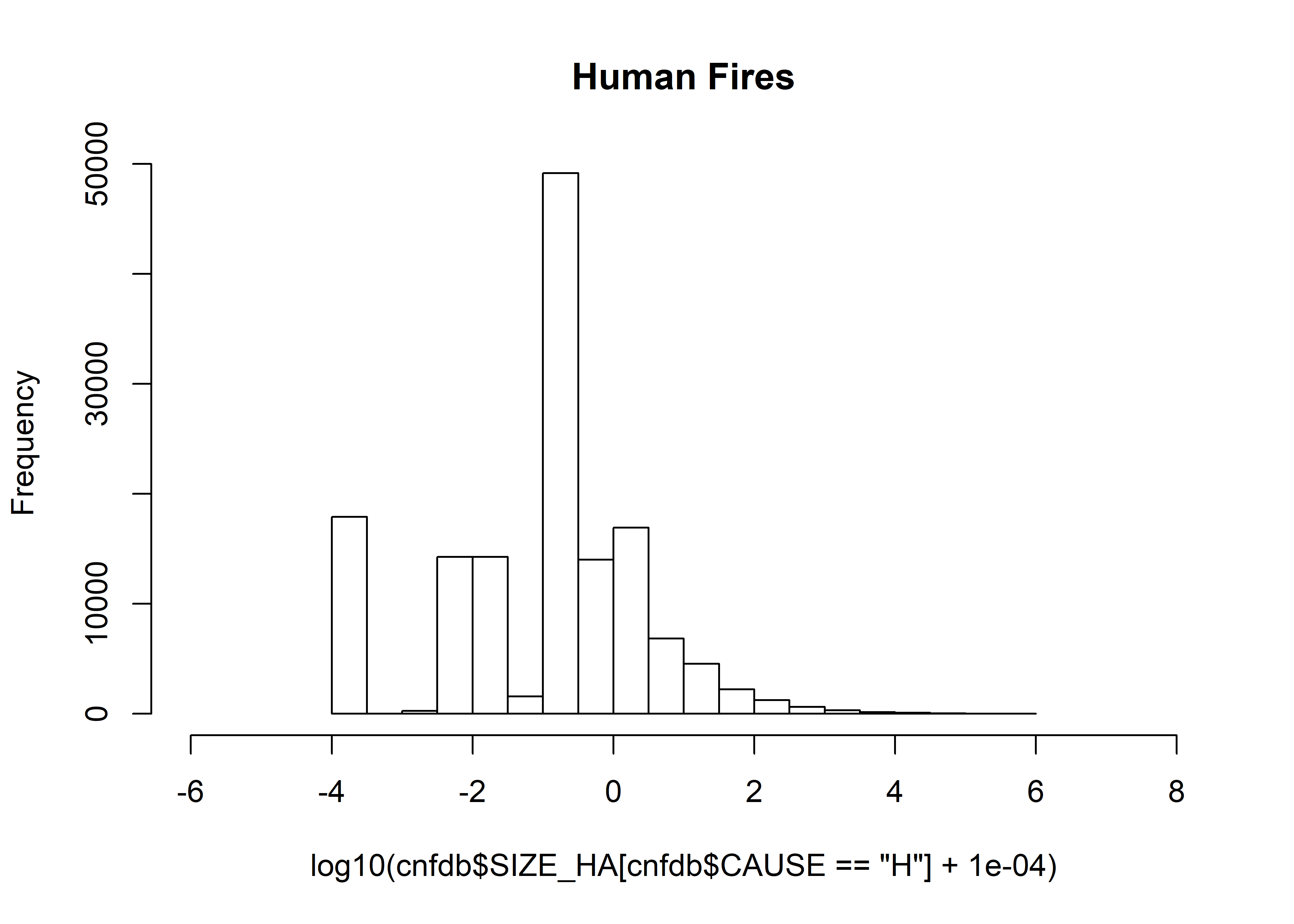
hist(log10(cnfdb$SIZE_HA[cnfdb$CAUSE == "L"]+0.0001), xlim=c(-6,8), breaks=20,
  main="Lightning Fires")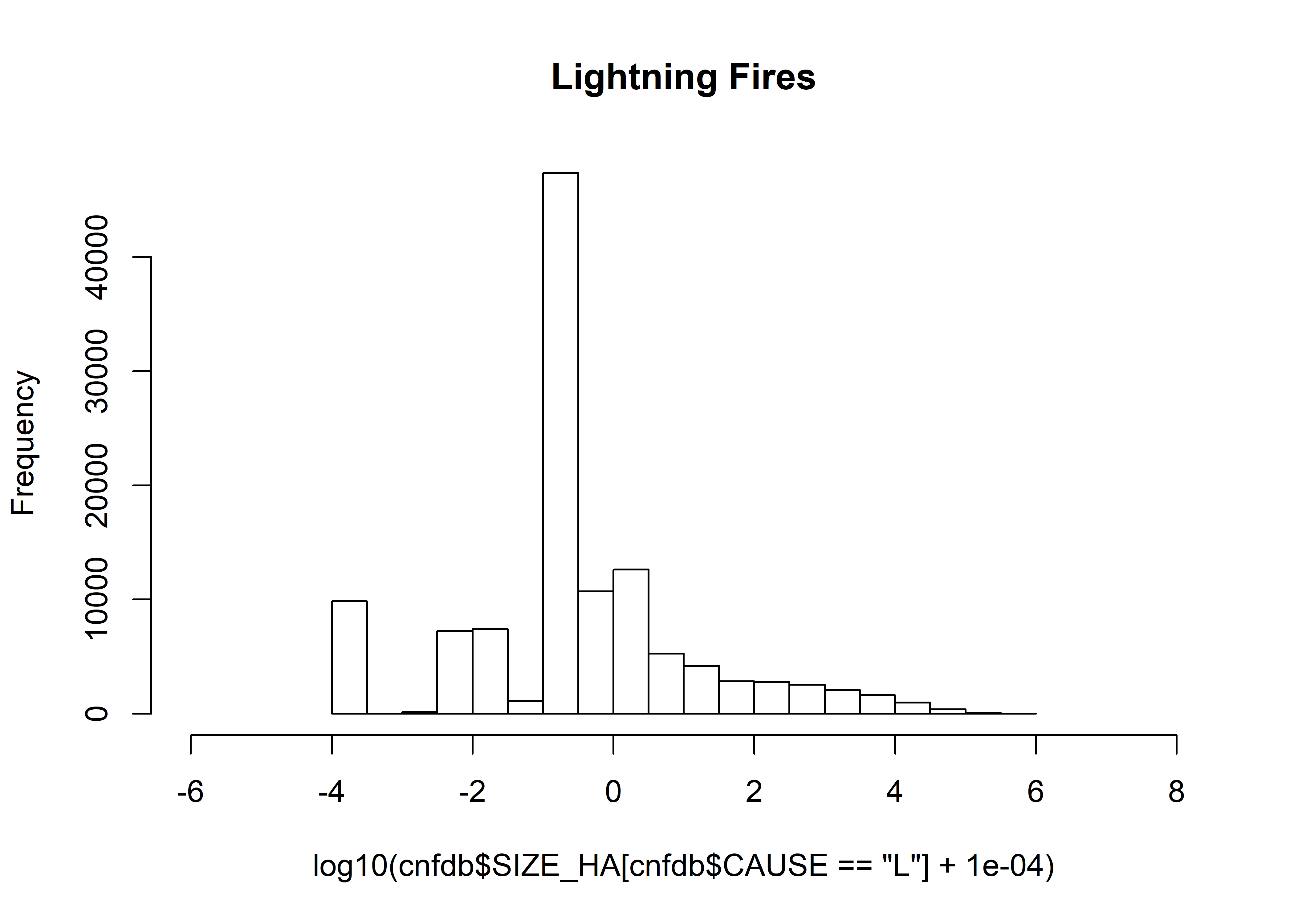
1.3.3 Mosaic plots
Mosaic plots, by month and year.
cnfdb.tablemon <- table(cnfdb$YEAR, cnfdb$startmon)
mosaicplot(cnfdb.tablemon, color=monthcolors, cex.axis=0.6, las=3, main="All Fires")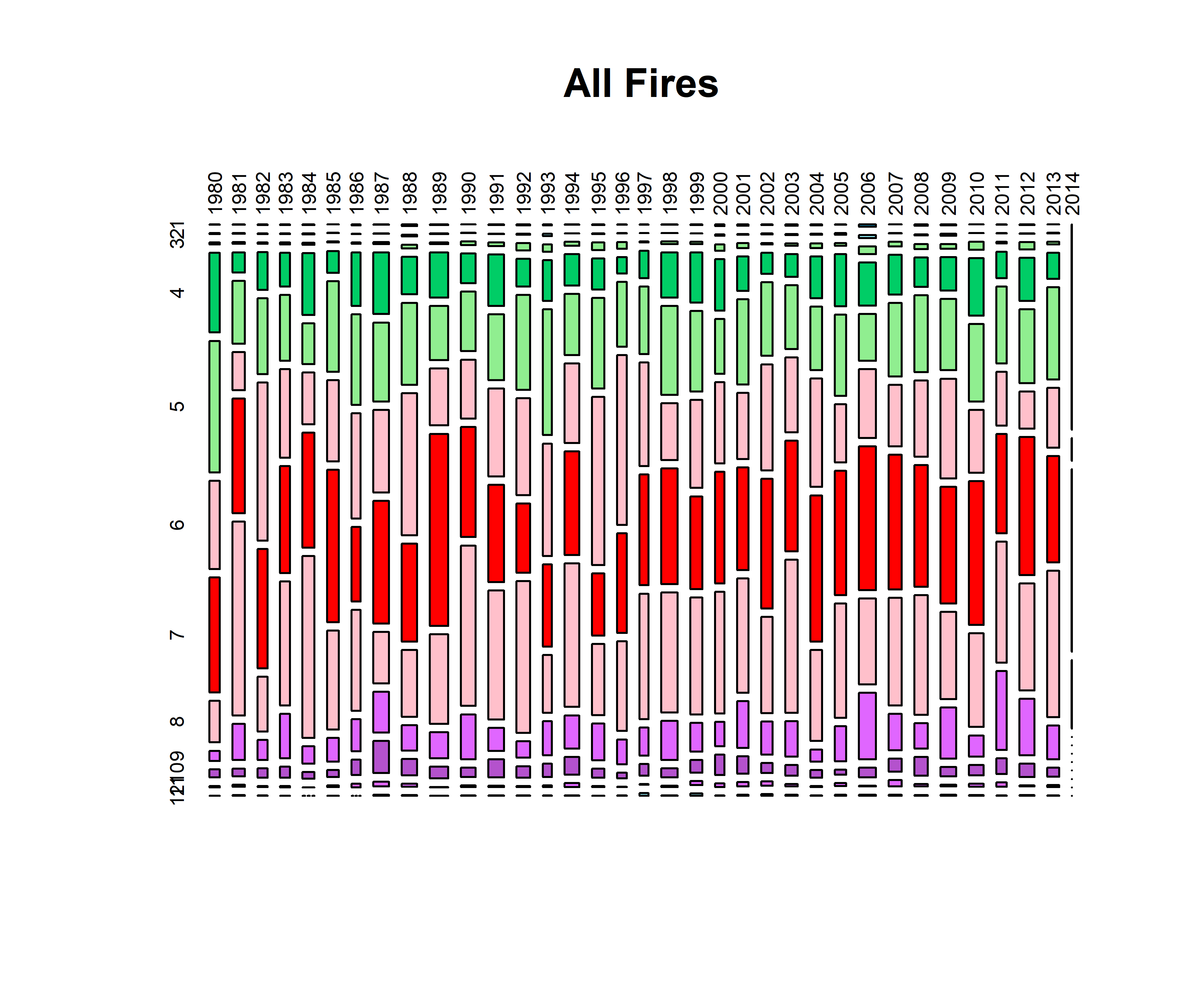
cnfdb.tablemon.h <- table(cnfdb$YEAR[cnfdb$CAUSE=="H"], cnfdb$startmon[cnfdb$CAUSE=="H"])
mosaicplot(cnfdb.tablemon.h, color=monthcolors, cex.axis=0.6, las=3, main="Human Fires")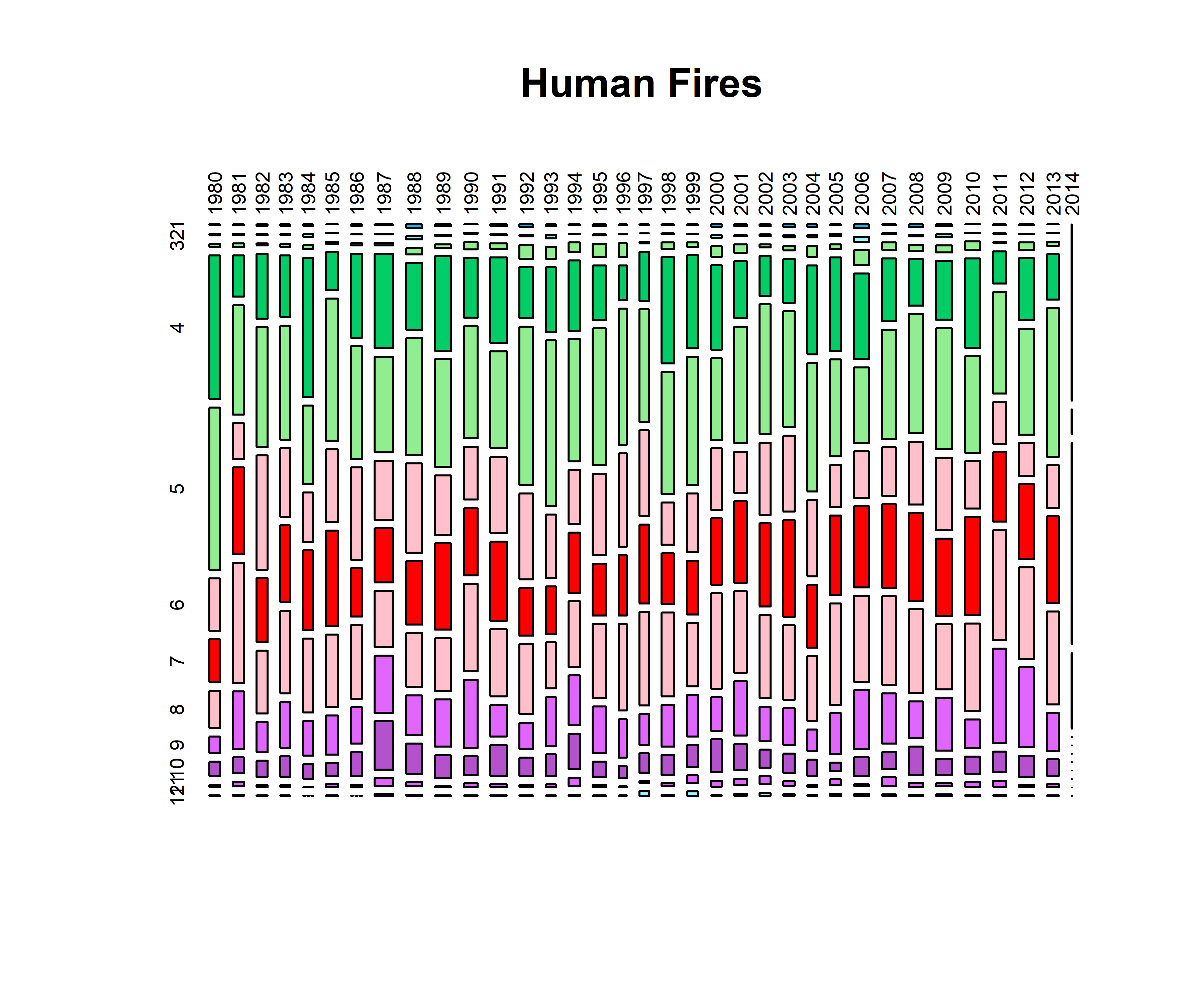
cnfdb.tablemon.n <- table(cnfdb$YEAR[cnfdb$CAUSE=="L"], cnfdb$startmon[cnfdb$CAUSE=="L"])
mosaicplot(cnfdb.tablemon.n, color=monthcolors, cex.axis=0.6, las=3, main="Lightning Fires")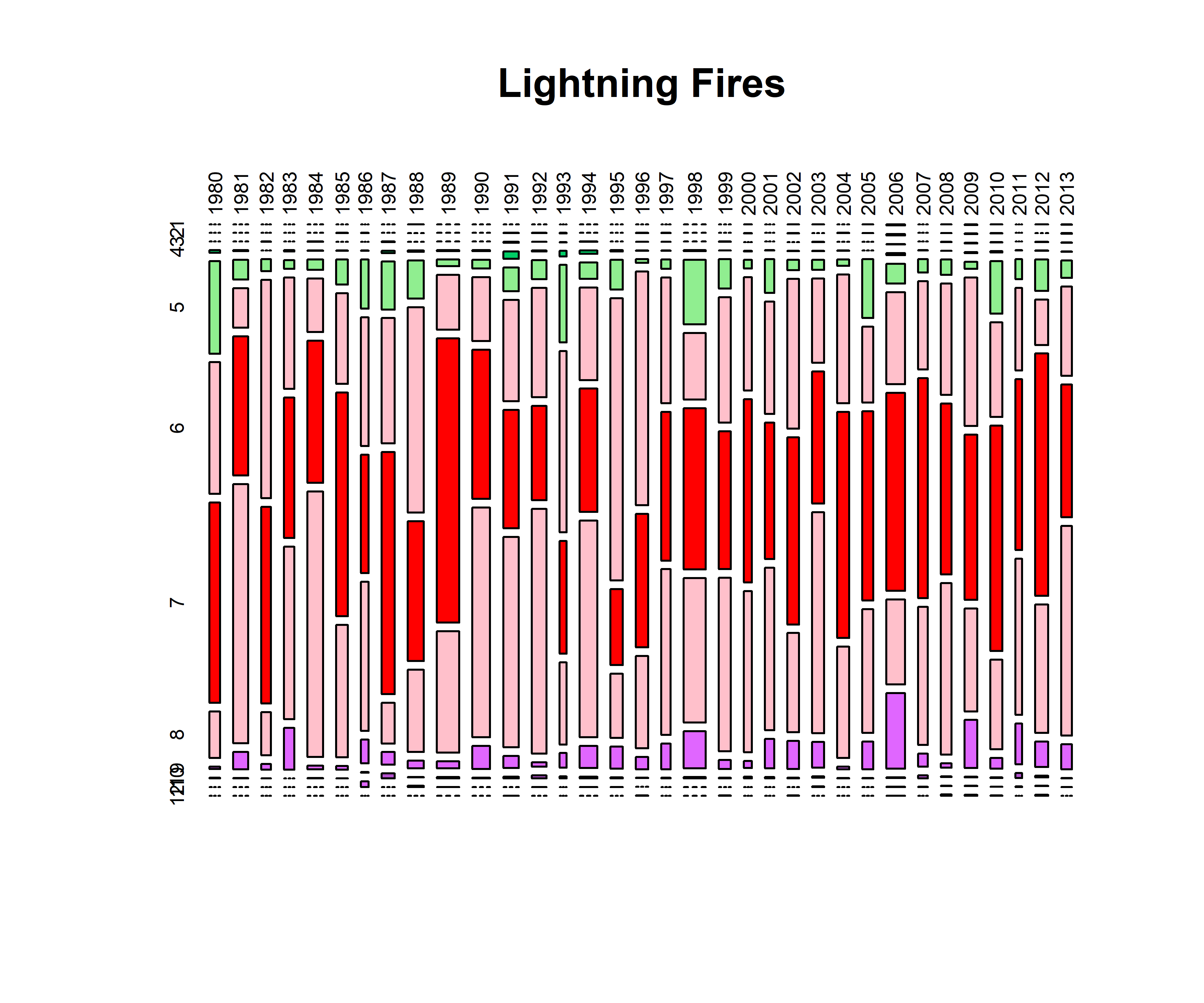
cnfdb.tablecause <- table(cnfdb$YEAR, cnfdb$agency)
mosaicplot(cnfdb.tablecause, cex.axis=0.6, las=2, color=mosaiccolor, main="Fires by Agency")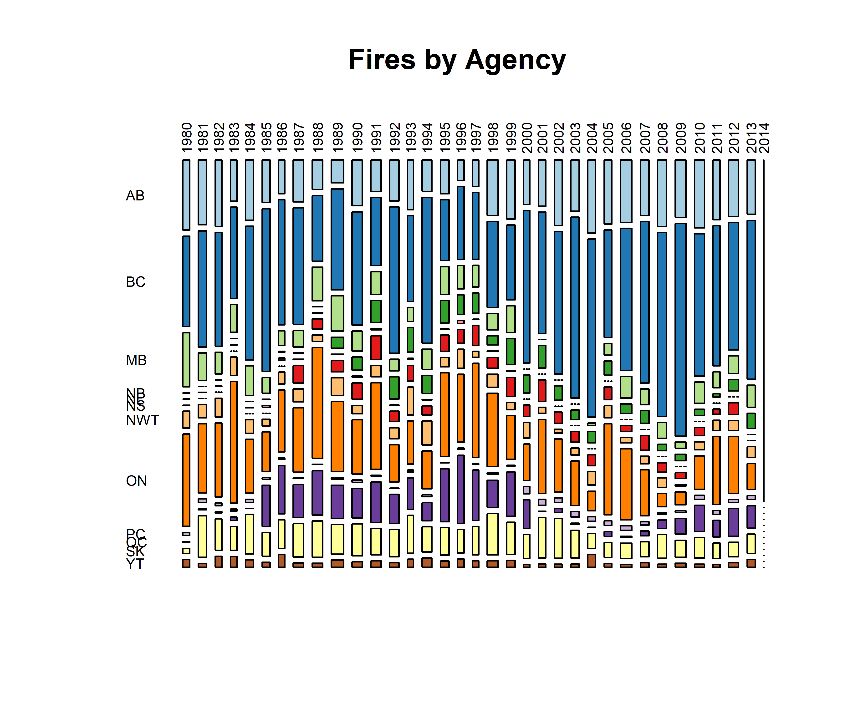
cnfdb.tablecause <- table(cnfdb$YEAR, cnfdb$CAUSE)
mosaicplot(cnfdb.tablecause, cex.axis=0.6, las=2, color=mosaiccolor, main="Fires by Cause")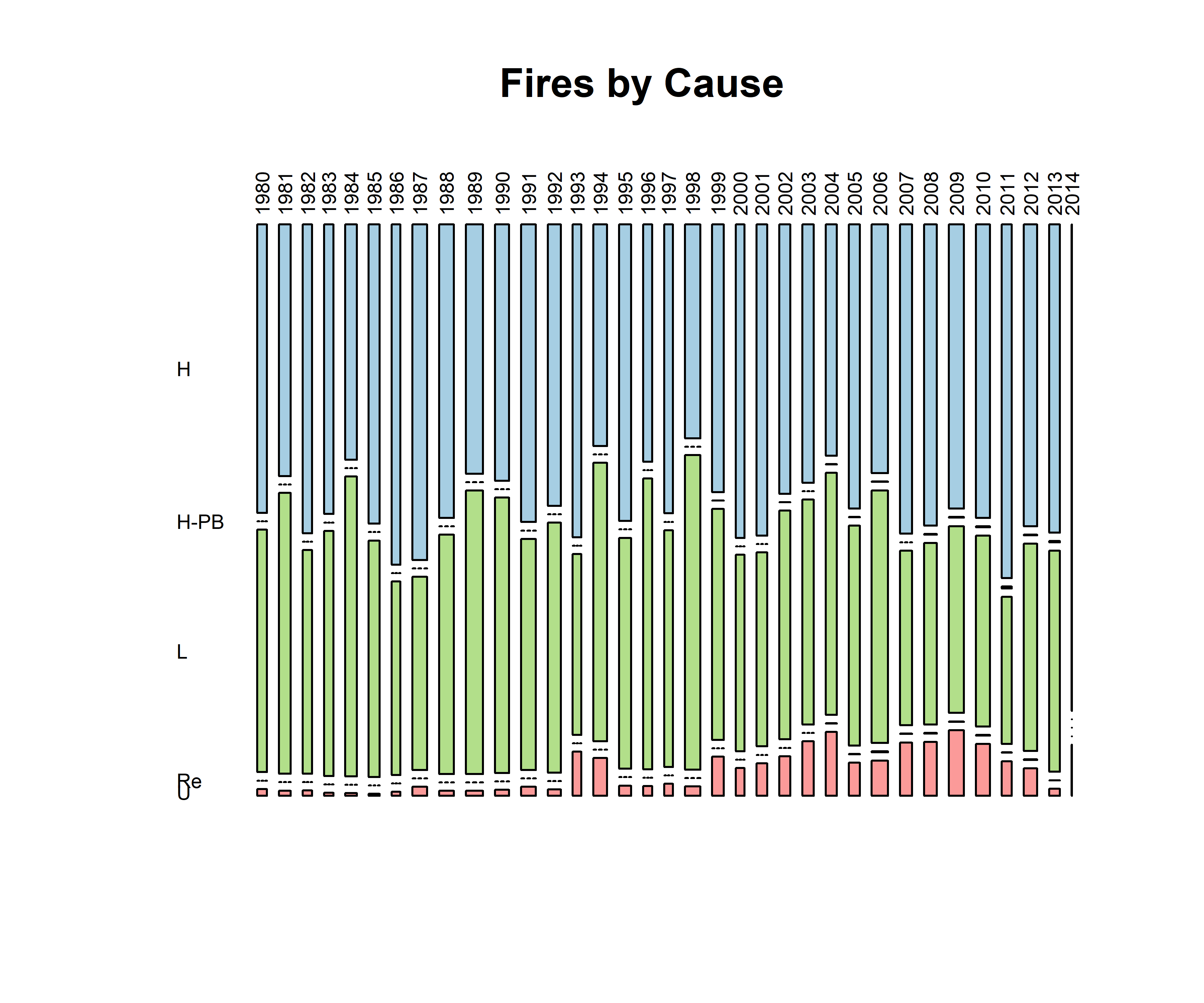
cnfdb.tableagencycause <- table(cnfdb$agency, cnfdb$CAUSE)
mosaicplot(cnfdb.tableagencycause, cex.axis=0.6, las=2, color=mosaiccolor, main="Fires by Agency and Cause")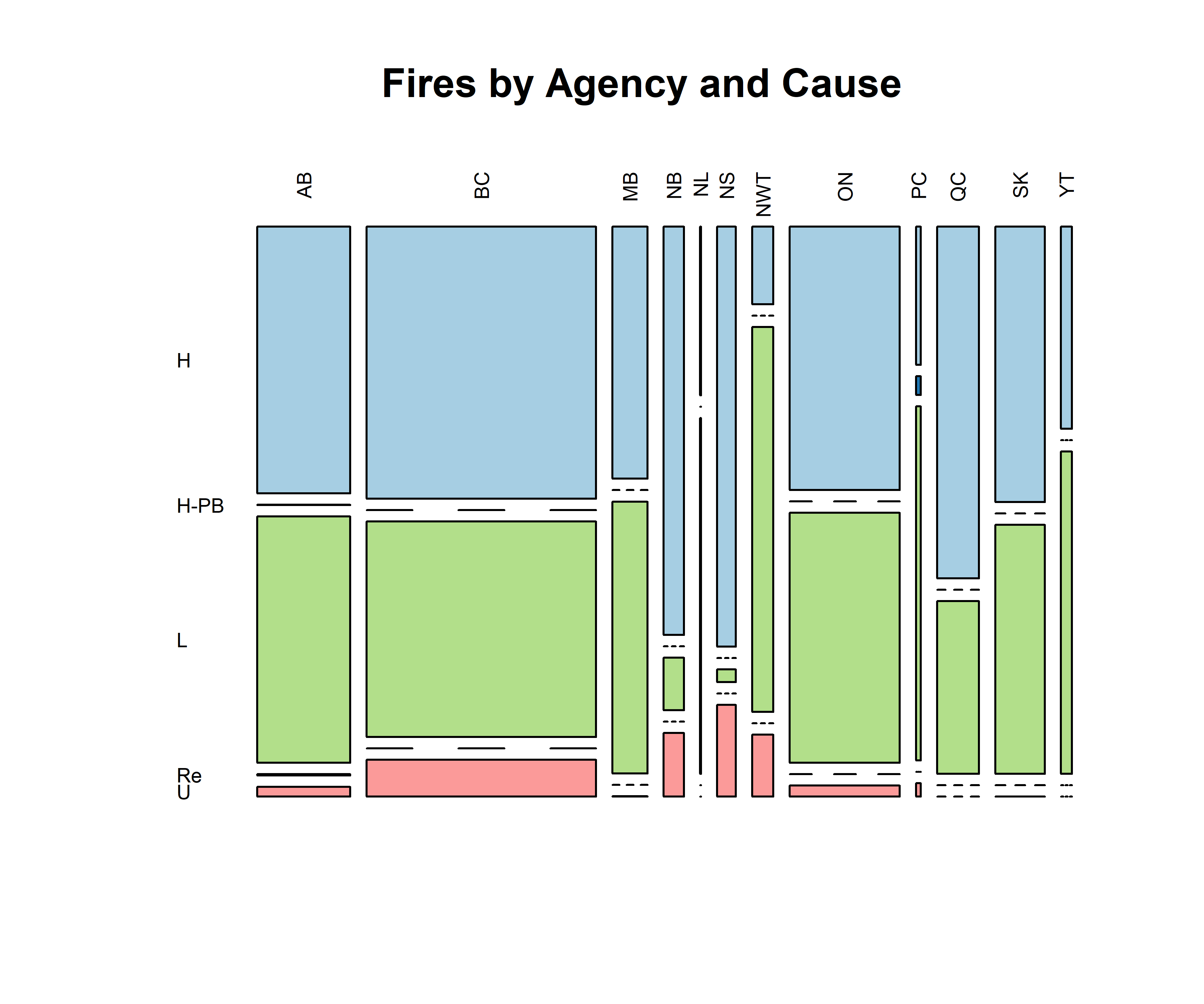
The mosaic plots suggest that the records are quite complete back to 1980 (except for 2014).