Intercomparison of U.S. Fire-Start Data Sets
1 Intercomparison of the FPA-FOD, FWFOD, and NIFC data sets
The objective of this analysis is to compare the three main U.S. data set, and evaluate the possibility of using the NIFC data set to exthen the FPA-FOD data set back into the 1980s. (Except for annually aggregated records, the FWFOD data set can not be used for that purpose, owing to the start-day problem in that data set.)
2 Data sets
Load the .RData versions of the cleaned up data sets. (These were saved during the analyses of the individual data sets.) (Note that for convenience, the “cleaned up” Canadian data set (cnfdb_v2) is also read in here.)
load("e:/Projects/fire/DailyFireStarts/data/RData/fpafod.RData")
load("e:/Projects/fire/DailyFireStarts/data/RData/fwfod.RData")
load("e:/Projects/fire/DailyFireStarts/data/RData/nifc.RData")
load("e:/Projects/fire/DailyFireStarts/data/RData/cnfdb_v2.RData")
Save the data as an .RData file:
save.image("e:/Projects/fire/DailyFireStarts/data/RData/alldb.RData")3 Compare FPA-FOD, FWFOD, and NIFC – All fires
For each data set, the number of fires each year and the total area and mean area burned are plotted for each year.
3.1 Maps
library(maps)
plot(fpafod$LATITUDE ~ fpafod$LONGITUDE, ylim=c(17,80), xlim=c(-180,-55), type="n",
  xlab="Longitude", ylab="Latitude", main="FPA-FOD -- All Fires")
map("world", add=TRUE, lwd=2, col="gray")
points(fpafod$LATITUDE ~ fpafod$LONGITUDE, pch=16, cex=0.2, col="red")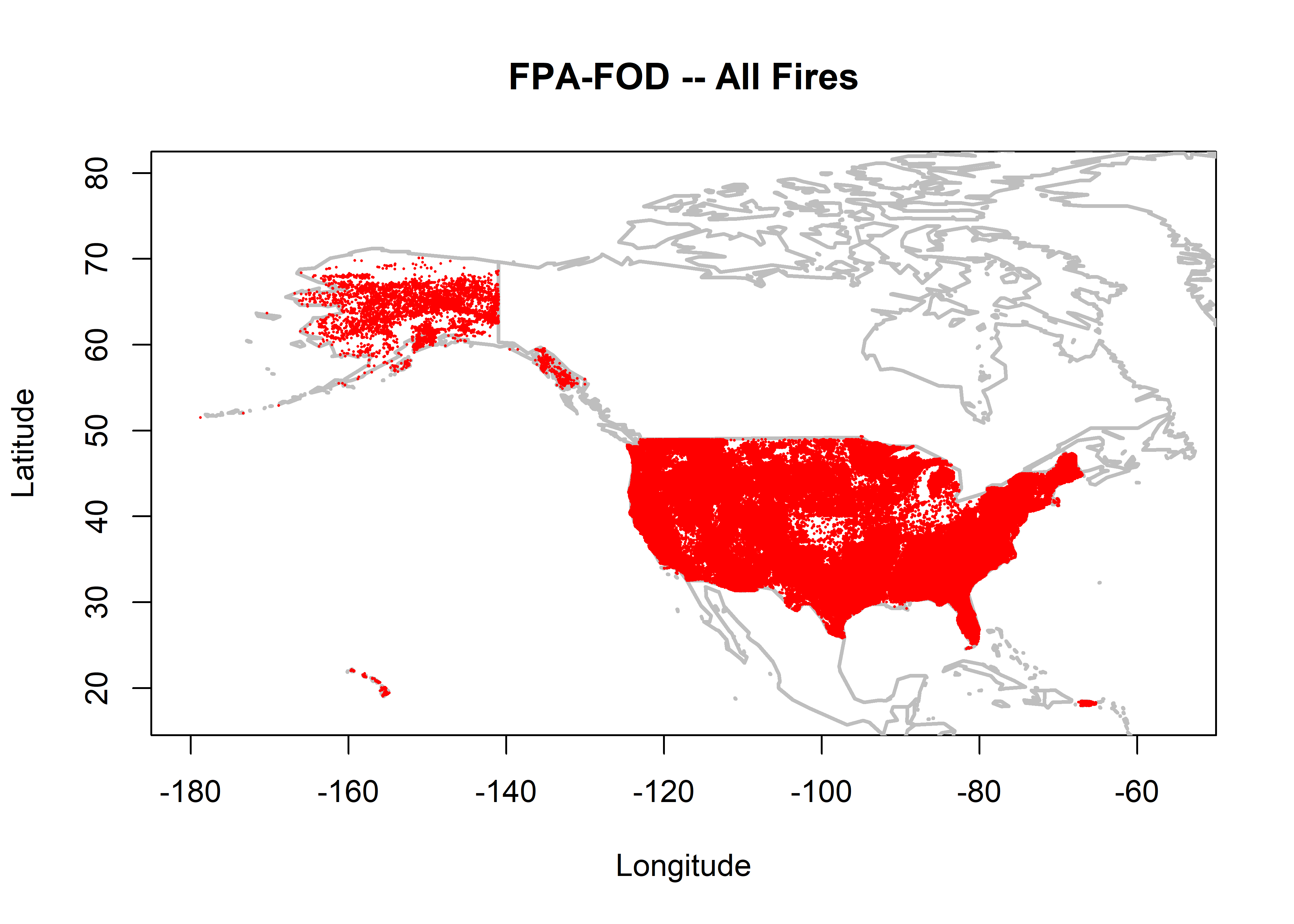
plot(nifc$LATITUDE ~ nifc$LONGITUDE, ylim=c(17,80), xlim=c(-180,-55), type="n",
  xlab="Longitude", ylab="Latitude", main="NIFC -- All Fires")
map("world", add=TRUE, lwd=2, col="gray")
points(nifc$LATITUDE ~ nifc$LONGITUDE, pch=16, cex=0.2, col="red")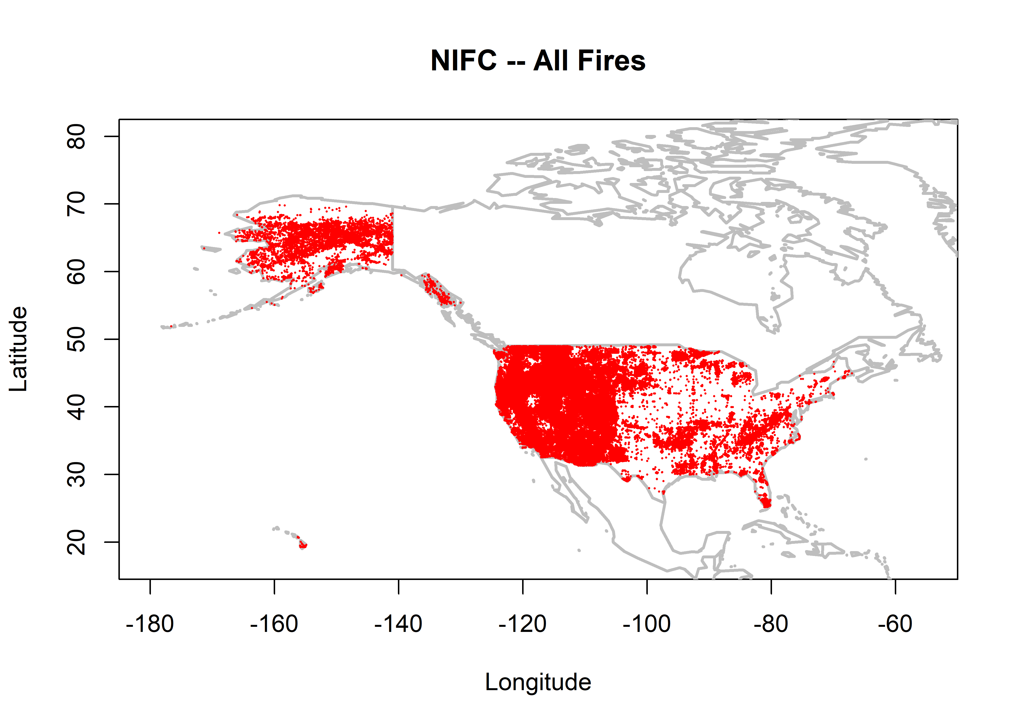
plot(fwfod$DLATITUDE ~ fwfod$DLONGITUDE, ylim=c(17,80), xlim=c(-180,-55), type="n",
  xlab="Longitude", ylab="Latitude", main="FWFOD -- All Fires")
map("world", add=TRUE, lwd=2, col="gray")
points(fwfod$DLATITUDE ~ fwfod$DLONGITUDE, pch=16, cex=0.2, col="red")
It can be easily seen that the FPA-FOD data set has the most dense spatial coverage, and the NIFC data set the least. However, all of the data sets have similar density of coverage in the western U.S. and Alaska.
3.2 Time series – number and area
3.2.1 Total number of fires
Get the number of fires each year for each data set, and make a data frame for plotting.
fpafod_num <- hist(fpafod$FIRE_YEAR, breaks=seq(1979.5,2015.5, by=1), plot = FALSE)
nifc_num <- hist(nifc$YEAR, breaks=seq(1979.5,2015.5, by=1), plot = FALSE)
fwfod_num <- hist(fwfod$startyear, breaks=seq(1979.5,2015.5,by=1), plot = FALSE)

all_num <- data.frame(fpafod_num$mids, fpafod_num$counts, nifc_num$counts, fwfod_num$counts)
all_num[all_num == 0] <- NA
names(all_num) <- c("Year", "fpafod_num", "nifc_num", "fwfod_num")
all_num
## Year fpafod_num nifc_num fwfod_num
## 1 1980 NA NA 8954
## 2 1981 NA 5470 10328
## 3 1982 NA 3622 6278
## 4 1983 NA 4962 6451
## 5 1984 NA 6223 9147
## 6 1985 NA 8172 10390
## 7 1986 NA 17760 15489
## 8 1987 NA 21873 19422
## 9 1988 NA 21950 19908
## 10 1989 NA 19857 17797
## 11 1990 NA 20606 17830
## 12 1991 NA 19530 17332
## 13 1992 67964 22266 19320
## 14 1993 62022 17025 14300
## 15 1994 75989 27081 23666
## 16 1995 71496 19560 16754
## 17 1996 75604 23273 20189
## 18 1997 61472 16280 14309
## 19 1998 68388 19524 18183
## 20 1999 89398 21726 21657
## 21 2000 96454 23975 23064
## 22 2001 86069 22581 21303
## 23 2002 75136 21545 20639
## 24 2003 67380 20075 22155
## 25 2004 68616 NA 19210
## 26 2005 87391 NA 19508
## 27 2006 113242 NA 24576
## 28 2007 94681 NA 20414
## 29 2008 84654 NA 15651
## 30 2009 77262 NA 15742
## 31 2010 78485 NA 14946
## 32 2011 89897 NA 15801
## 33 2012 71768 NA 16320
## 34 2013 64108 NA 16380
## 35 2014 NA NA 15475
## 36 2015 NA NA NATime series plots of the numbers of fires:
plot(all_num$fpafod_num ~ all_num$Year, type="o", col="red", pch=16, xlim=c(1980,2015), ylim=c(0,120000),
  xlab="Year", ylab="Total Number of Fires", main="Total Number of Fires (U.S. All)", lwd=2)
lines(all_num$nifc_num ~ all_num$Year, type="o", col="blue", pch=16, lwd=2)
lines(all_num$fwfod_num ~ all_num$Year, type="o", col="purple", pch=16, lwd=2)
legend("topleft", legend=c("FPA-FOD","NIFC","FWFOD"), lwd=2, col=c("red","blue","purple"))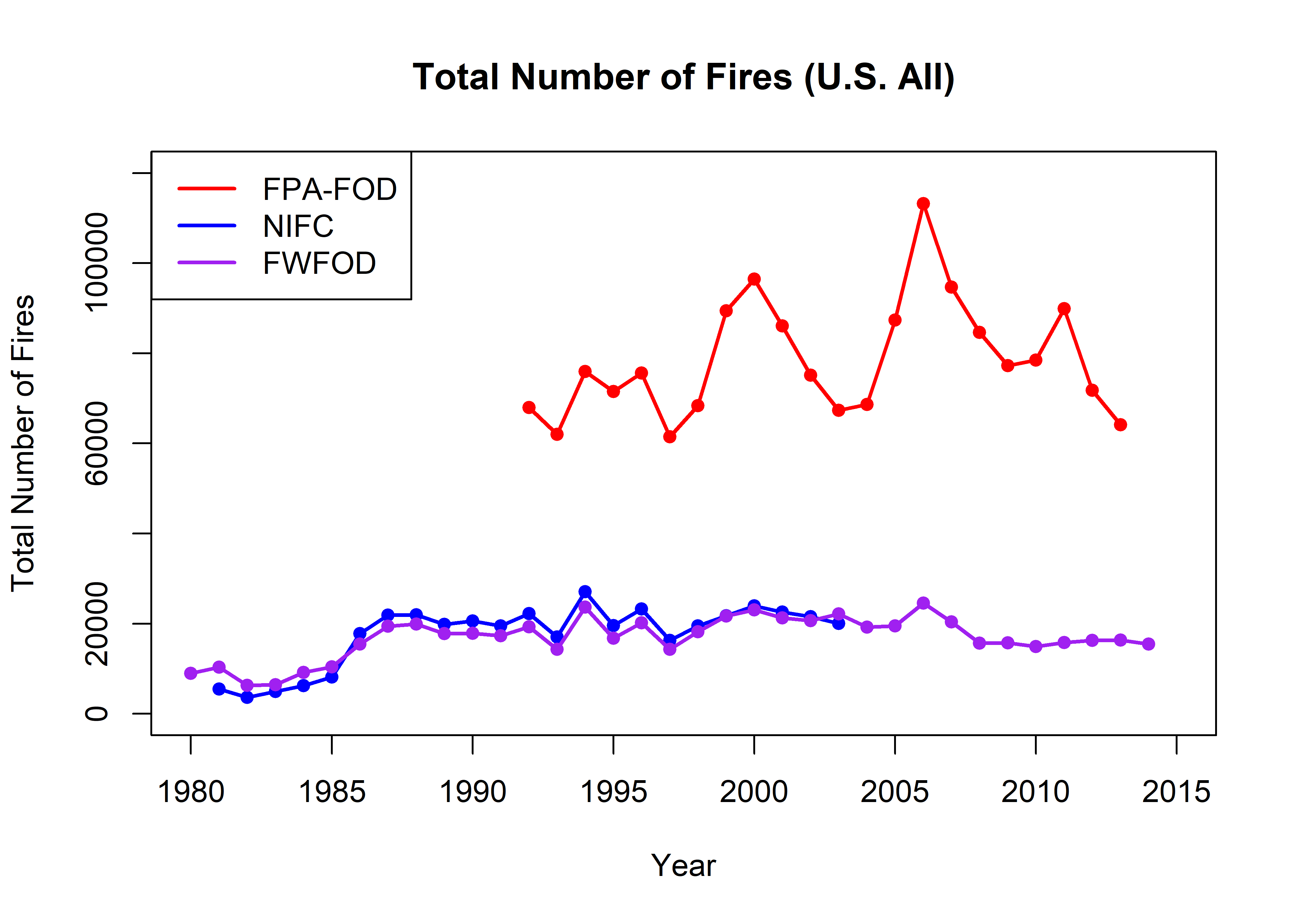
Scatter plots that compare the three different data sets:
oldpar <- par(mfrow=c(1,3))
plot(all_num$fpafod_num, all_num$nifc_num, xlim=c(0,120000), ylim=c(0,120000), pch=16, xlab="FPA-FOD",
     ylab="NIFC"); abline(0,1); abline(0,1)
plot(all_num$fpafod_num, all_num$fwfod_num, xlim=c(0,120000), ylim=c(0,120000), pch=16, xlab="FPA-FOD",
     ylab="FWFOD", main="Total Number of Fires"); abline(0,1)
plot(all_num$fwfod_num, all_num$nifc_num, xlim=c(0,120000), ylim=c(0,120000), pch=16, xlab="FWFOD",
     ylab="NIFC"); abline(0,1)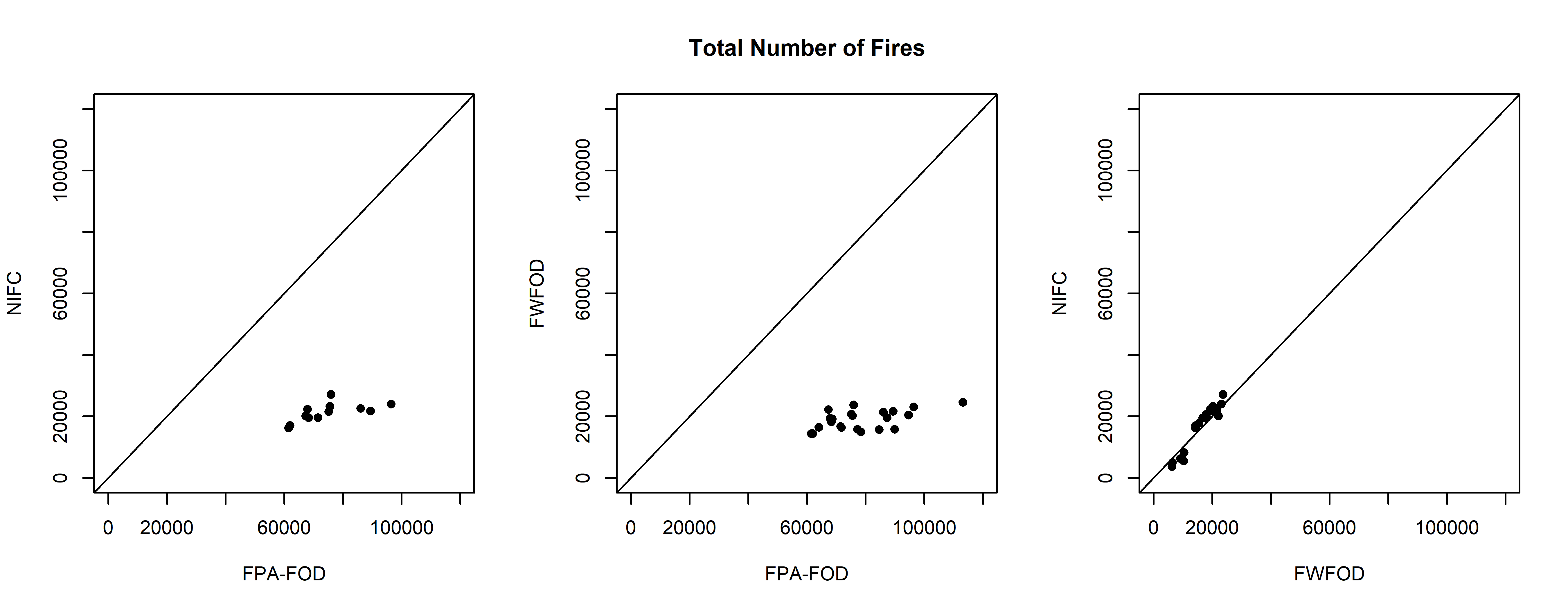
par(oldpar)The FPA-FOD data set can clearly be seen to have many more fires per year than the FWFOD and NIFC data sets, and the FPA-FOD also shows larger-amplitude interannual variability. As will be discussed further below, this can be attributed to the greater number of human-started fires in the FPA-FOD data set. When they overlap, the NIFC and FWFOD data sets are highly correlated (r = 0.9626519)
3.2.2 Total area burned
Get time series of total area burned.
all_totalarea <- data.frame(matrix(nrow = 36, ncol = 4))
names(all_totalarea) <- c("Year", "fpafod_totalarea", "nifc_totalarea", "fwfod_totalarea")
all_totalarea["Year"] <- seq(1980, 2015, by=1)

fpafod_total_by_year <- tapply(fpafod$AREA_HA, fpafod$FIRE_YEAR, sum)
fpafod_year <- as.numeric(unlist(dimnames(fpafod_total_by_year)))
fpafod_total_by_year <- as.numeric(fpafod_total_by_year)
all_totalarea$fpafod_totalarea[fpafod_year-1980+1] <- fpafod_total_by_year

fwfod_total_by_year <- tapply(fwfod$AREA, fwfod$startyear, sum)
fwfod_year <- as.numeric(unlist(dimnames(fwfod_total_by_year)))
fwfod_total_by_year <- as.numeric(fwfod_total_by_year)
all_totalarea$fwfod_totalarea[fwfod_year-1980+1] <- fwfod_total_by_year

nifc_size_year <- na.omit(cbind(nifc$AREA,nifc$YEAR))
nifc_total_by_year <- tapply(nifc_size_year[,1],nifc_size_year[,2], sum)
nifc_year <- as.numeric(unlist(dimnames(nifc_total_by_year)))
nifc_total_by_year <- as.numeric(nifc_total_by_year)
all_totalarea$nifc_totalarea[nifc_year-1980+1] <- nifc_total_by_year

all_totalarea
## Year fpafod_totalarea nifc_totalarea fwfod_totalarea
## 1 1980 NA NA 376937.7
## 2 1981 NA 761623.3 772901.1
## 3 1982 NA 161606.7 174664.0
## 4 1983 NA 491391.3 272892.2
## 5 1984 NA 569117.8 496682.0
## 6 1985 NA 866913.3 888544.9
## 7 1986 NA 890000.7 619901.7
## 8 1987 NA 1008909.0 951178.4
## 9 1988 NA 3234560.1 3771214.7
## 10 1989 NA 609348.5 610271.2
## 11 1990 NA 1878924.3 1610359.9
## 12 1991 NA 953758.2 1142398.2
## 13 1992 889967.4 753982.3 606096.8
## 14 1993 886494.5 648430.7 759900.1
## 15 1994 1666373.0 1400158.2 1323328.4
## 16 1995 829494.6 588081.4 483741.4
## 17 1996 2430644.9 2088975.6 1966609.8
## 18 1997 1301188.9 1057420.0 1077143.9
## 19 1998 806010.4 501125.5 437718.8
## 20 1999 2455889.8 2066090.8 1983707.5
## 21 2000 3090726.6 2714832.3 3290616.5
## 22 2001 1506323.0 1214376.3 897304.4
## 23 2002 2752402.0 2984240.6 3768737.2
## 24 2003 1810067.0 1809037.8 1891143.8
## 25 2004 3331301.4 NA 3970058.5
## 26 2005 3901577.5 NA 5129648.1
## 27 2006 4062770.0 NA 2997866.5
## 28 2007 3748792.6 NA 3150657.8
## 29 2008 2187148.7 NA 1353575.6
## 30 2009 2449661.4 NA 2421749.2
## 31 2010 1411129.9 NA 1213475.7
## 32 2011 3891441.7 NA 1882140.1
## 33 2012 3820172.7 NA 2818741.0
## 34 2013 1816678.9 NA 1762509.8
## 35 2014 NA NA 1368776.7
## 36 2015 NA NA NAPlot the time series of total area burned:
plot(all_totalarea$fpafod_totalarea ~ all_totalarea$Year, type="o", col="red", pch=16, lwd=2, xlim=c(1980,2015), ylim=c(0,6000000),
  xlab="Year", ylab="Total Area Burned", main="Total Area Burned (ha) (U.S. All)")
points(all_totalarea$fwfod_totalarea ~ all_totalarea$Year, type="o", col="purple", pch=16, lwd=2)
points(all_totalarea$nifc_totalarea ~ all_totalarea$Year, type="o", col="blue", pch=16, lwd=2)
legend("topleft", legend=c("FPA-FOD","NIFC","FWFOD"), lwd=2, col=c("red","blue","purple"))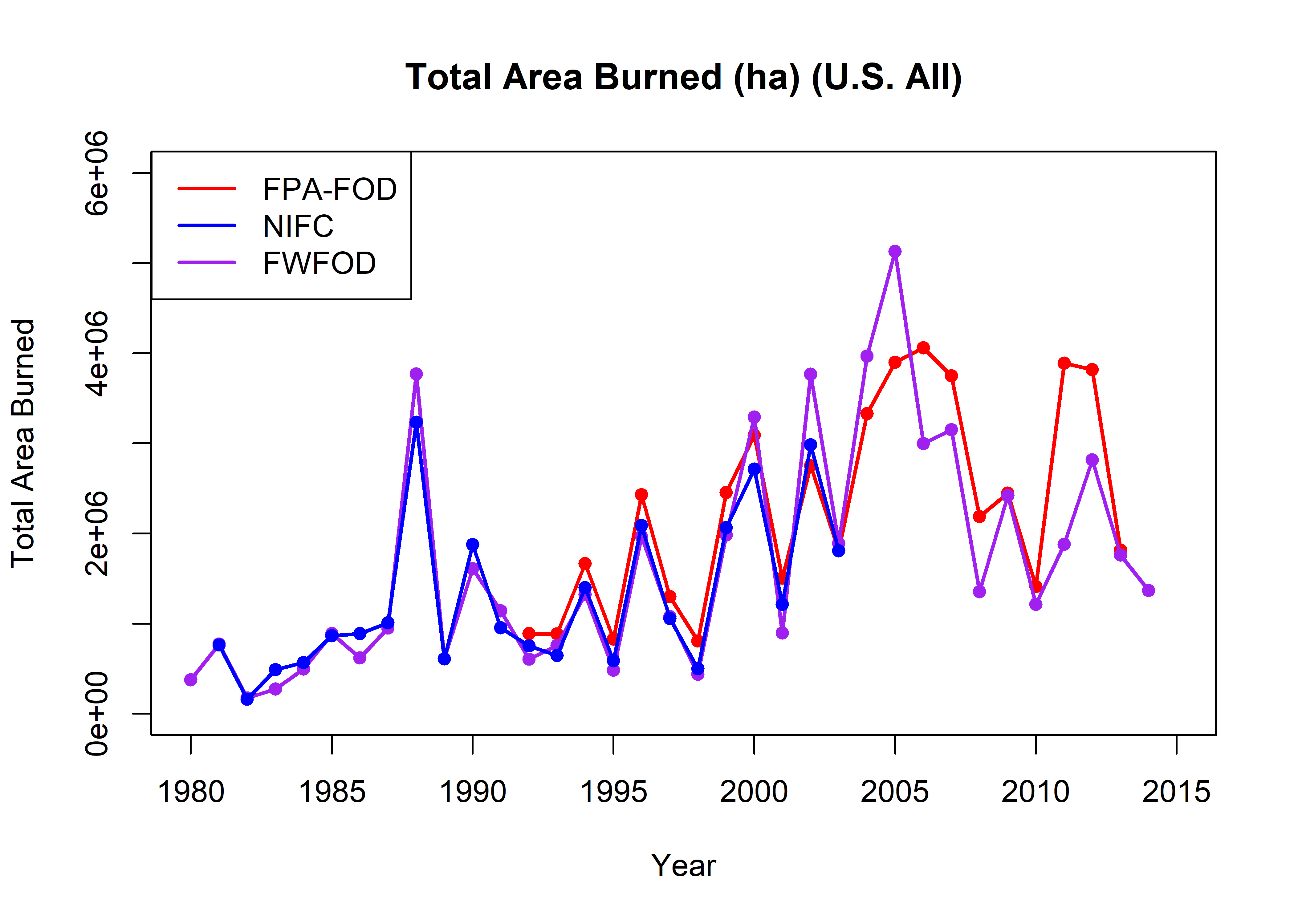
When the series overlap, the total areas burned in each data set are quite similar, more similar in character than the total number of fires. This implies again that many of the “additional” fires in the FPA-FOD data set are small fires. Note that quite similar before then, the FPA-FOD and FWFOD diverge somewhat in 2005 and thereafter.
Scatter plots of the total areas burned in each data set:
oldpar <- par(mfrow=c(1,3))
plot(all_totalarea$fpafod_totalarea, all_totalarea$nifc_totalarea, xlim=c(0,6000000), ylim=c(0,6000000),
     pch=16, xlab="FPA-FOD", ylab="NIFC"); abline(0,1)
plot(all_totalarea$fpafod_totalarea, all_totalarea$fwfod_totalarea, xlim=c(0,6000000), ylim=c(0,6000000),
     pch=16, xlab="FPA-FOD", ylab="FWFOD", main="Total Area Burned (ha) (U.S. All)"); abline(0,1)
plot(all_totalarea$fwfod_totalarea, all_totalarea$nifc_totalarea, xlim=c(0,6000000), ylim=c(0,6000000),
     pch=16, xlab="FWFOD", ylab="NIFC"); abline(0,1)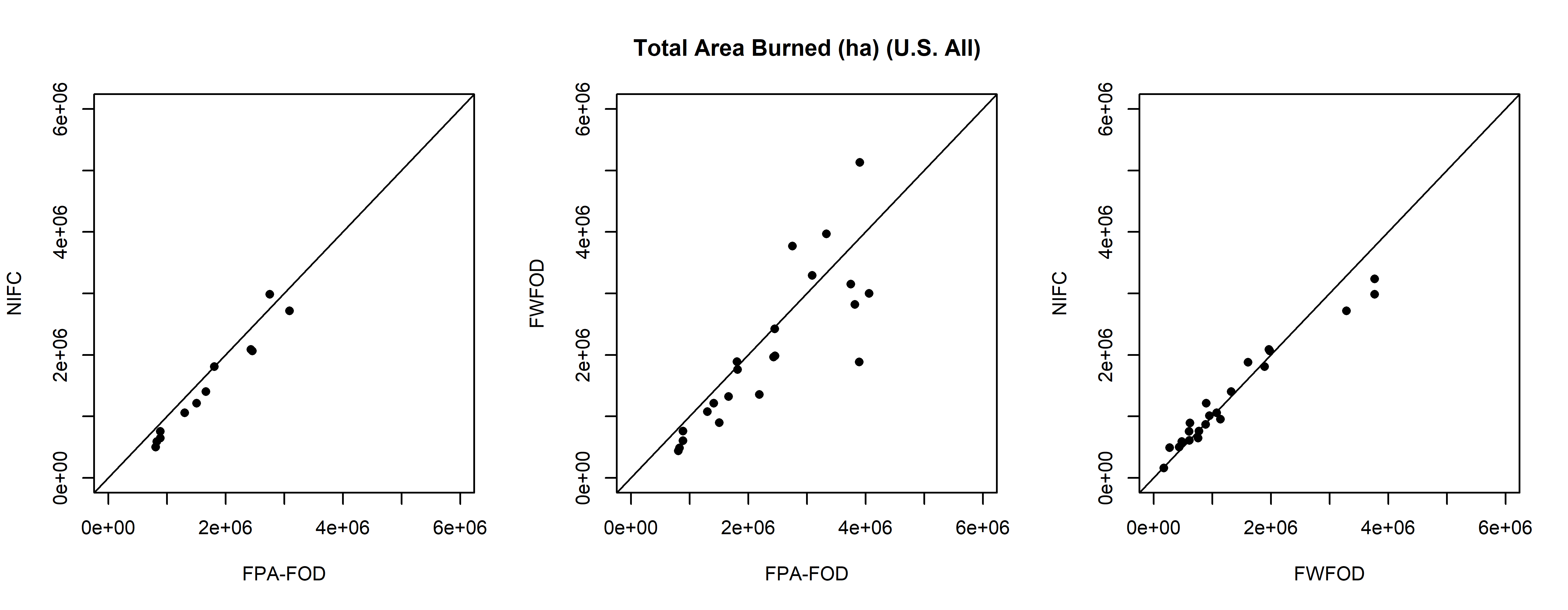
par(oldpar)Overall, there is more apparent agreement among data sets in the mean area burned each year than in the total number of fires. (See below.)
3.2.3 Mean area burned
all_meanarea <- data.frame(matrix(nrow = 36, ncol = 4))
names(all_meanarea) <- c("Year", "fpafod_meanarea", "nifc_meanarea", "fwfod_meanarea")
all_meanarea["Year"] <- seq(1980, 2015, by=1)

fpafod_mean_by_year <- tapply(fpafod$AREA_HA, fpafod$FIRE_YEAR, mean)
fpafod_year <- as.numeric(unlist(dimnames(fpafod_mean_by_year)))
fpafod_mean_by_year <- as.numeric(fpafod_mean_by_year)
all_meanarea$fpafod_meanarea[fpafod_year-1980+1] <- fpafod_mean_by_year

fwfod_mean_by_year <- tapply(fwfod$AREA, fwfod$startyear, mean)
fwfod_year <- as.numeric(unlist(dimnames(fwfod_mean_by_year)))
fwfod_mean_by_year <- as.numeric(fwfod_mean_by_year)
all_meanarea$fwfod_meanarea[fwfod_year-1980+1] <- fwfod_mean_by_year

nifc_size_year <- na.omit(cbind(nifc$AREA,nifc$YEAR))
nifc_mean_by_year <- tapply(nifc_size_year[,1],nifc_size_year[,2], mean)
nifc_year <- as.numeric(unlist(dimnames(nifc_mean_by_year)))
nifc_mean_by_year <- as.numeric(nifc_mean_by_year)
all_meanarea$nifc_meanarea[nifc_year-1980+1] <- nifc_mean_by_year

all_meanarea
## Year fpafod_meanarea nifc_meanarea fwfod_meanarea
## 1 1980 NA NA 42.09713
## 2 1981 NA 139.23643 74.83550
## 3 1982 NA 44.61810 27.82160
## 4 1983 NA 99.03089 42.30230
## 5 1984 NA 91.45392 54.29999
## 6 1985 NA 106.08337 85.51924
## 7 1986 NA 50.11265 40.02206
## 8 1987 NA 46.12577 48.97428
## 9 1988 NA 147.36037 189.43212
## 10 1989 NA 30.68684 34.29068
## 11 1990 NA 91.18336 90.31744
## 12 1991 NA 48.83555 65.91266
## 13 1992 13.09469 33.86250 31.37147
## 14 1993 14.29323 38.08697 53.13987
## 15 1994 21.92913 51.70260 55.91686
## 16 1995 11.60197 30.06551 28.87319
## 17 1996 32.14969 89.75962 97.40997
## 18 1997 21.16718 64.95209 75.27737
## 19 1998 11.78585 25.66716 24.07297
## 20 1999 27.47142 95.09762 91.59660
## 21 2000 32.04353 113.23597 142.67328
## 22 2001 17.50134 53.77868 42.12103
## 23 2002 36.63227 138.51198 182.60270
## 24 2003 26.86357 90.11396 85.35968
## 25 2004 48.54992 NA 206.66624
## 26 2005 44.64507 NA 262.95100
## 27 2006 35.87688 NA 121.98350
## 28 2007 39.59393 NA 154.33809
## 29 2008 25.83633 NA 86.48493
## 30 2009 31.70590 NA 153.83999
## 31 2010 17.97961 NA 81.19067
## 32 2011 43.28778 NA 119.11525
## 33 2012 53.22947 NA 172.71697
## 34 2013 28.33779 NA 107.60133
## 35 2014 NA NA 88.45084
## 36 2015 NA NA NAplot(fpafod_mean_by_year ~ fpafod_year, type="o", col="red", pch=16, lwd=2, xlim=c(1980,2015), ylim=c(0,300),
xlab="Year", ylab="Mean Area Burned", main="Mean Area Burned (ha) (U.S. All")
points(fwfod_mean_by_year ~ fwfod_year, type="o", col="purple", pch=16, lwd=2)
points(nifc_mean_by_year ~ nifc_year, type="o", col="blue", pch=16, lwd=2)
legend("topleft", legend=c("FPA-FOD","NIFC","FWFOD"), lwd=2, col=c("red","blue","purple"))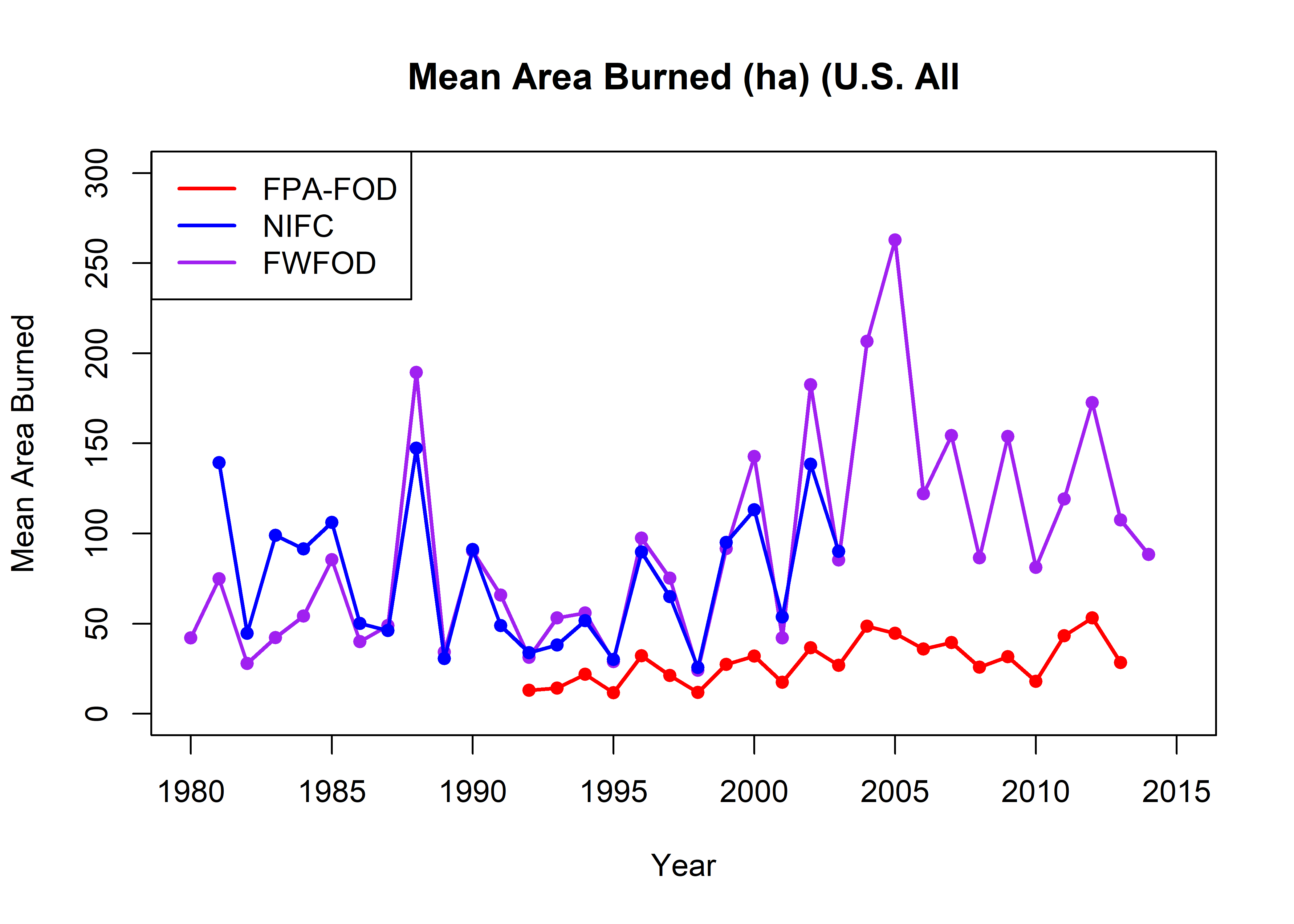
Scatter plots of the mean areas burned in each data set:
oldpar <- par(mfrow=c(1,3))
plot(all_meanarea$fpafod_meanarea, all_meanarea$nifc_meanarea, xlim=c(0,300), ylim=c(0,300),
     pch=16, xlab="FPA-FOD", ylab="NIFC"); abline(0,1)
plot(all_meanarea$fpafod_meanarea, all_meanarea$fwfod_meanarea, xlim=c(0,300), ylim=c(0,300),
     pch=16, xlab="FPA-FOD", ylab="FWFOD", main="Mean Area Burned (ha) (U.S. All)"); abline(0,1)
plot(all_meanarea$fwfod_meanarea, all_meanarea$nifc_meanarea, xlim=c(0,300), ylim=c(0,300 ),
     pch=16, xlab="FWFOD", ylab="NIFC"); abline(0,1)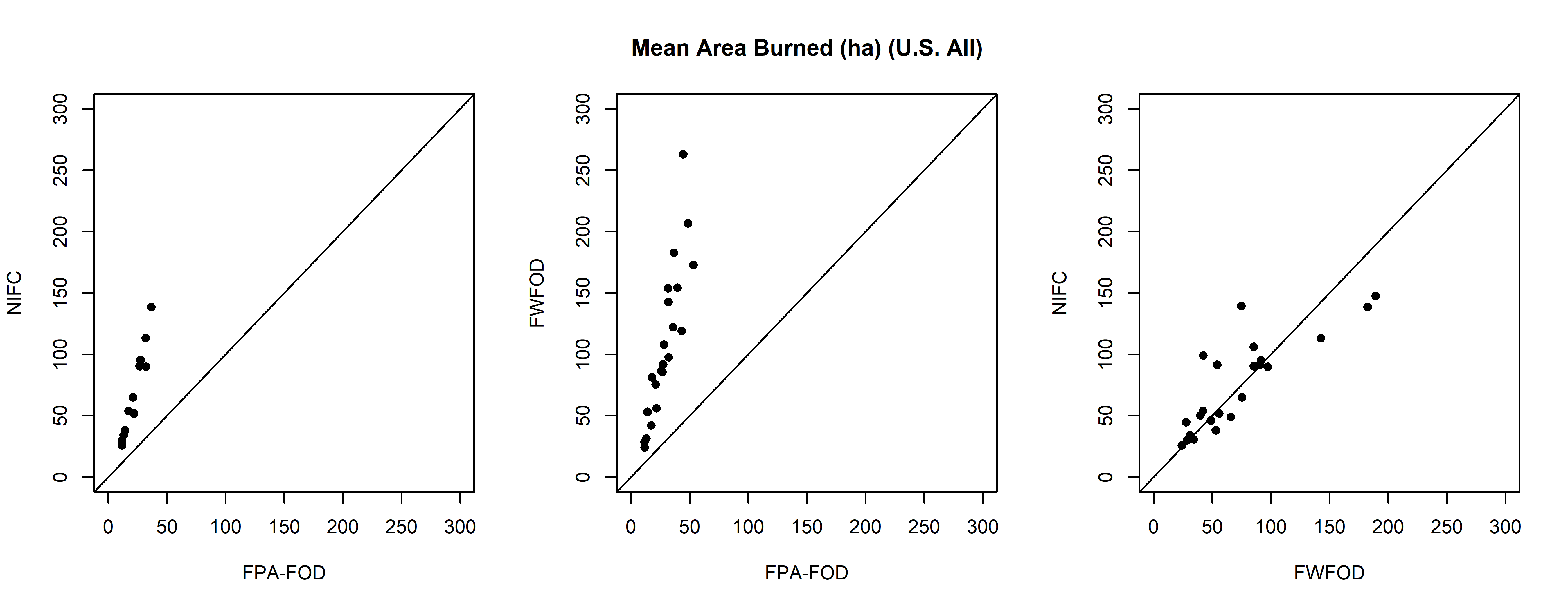
par(oldpar)3.3 Fire size class by year
sizecuts <- c(0.0,0.01,0.1,1,10,100,1000,10000) # c(0.0,0.00001,10,1000000) #
fpafod$sizeclass <- cut(fpafod$AREA_HA,sizecuts)
table(fpafod$sizeclass)
##
## (0,0.01] (0.01,0.1] (0.1,1] (1,10] (10,100] (100,1e+03] (1e+03,1e+04]
## 31743 520703 655620 378638 114084 21048 4777fpafod.tablesize <- table(fpafod$FIRE_YEAR, fpafod$sizeclass)
mosaicplot(fpafod.tablesize, color=TRUE, cex.axis=0.6, las=2, main="FPA-FOD by size (ha), All Fires")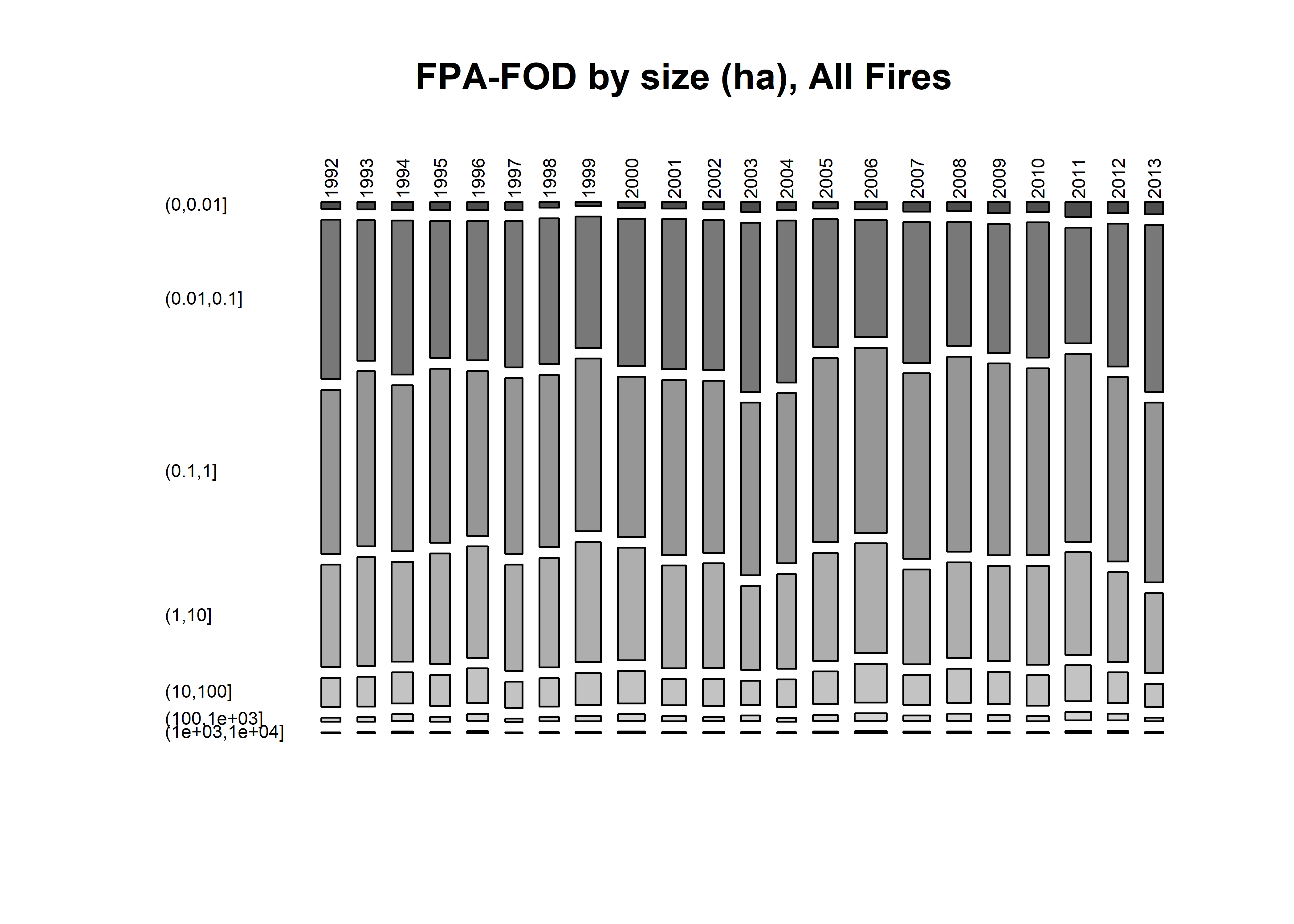
nifc$sizeclass <- cut(nifc$AREA,sizecuts)
table(nifc$sizeclass)
##
## (0,0.01] (0.01,0.1] (0.1,1] (1,10] (10,100] (100,1e+03] (1e+03,1e+04]
## 0 191454 95506 52210 25726 10111 3213nifc.tablesize <- table(nifc$YEAR, nifc$sizeclass)
mosaicplot(nifc.tablesize, color=TRUE, cex.axis=0.6, las=2, main="NIFC by size (ha), All Fires")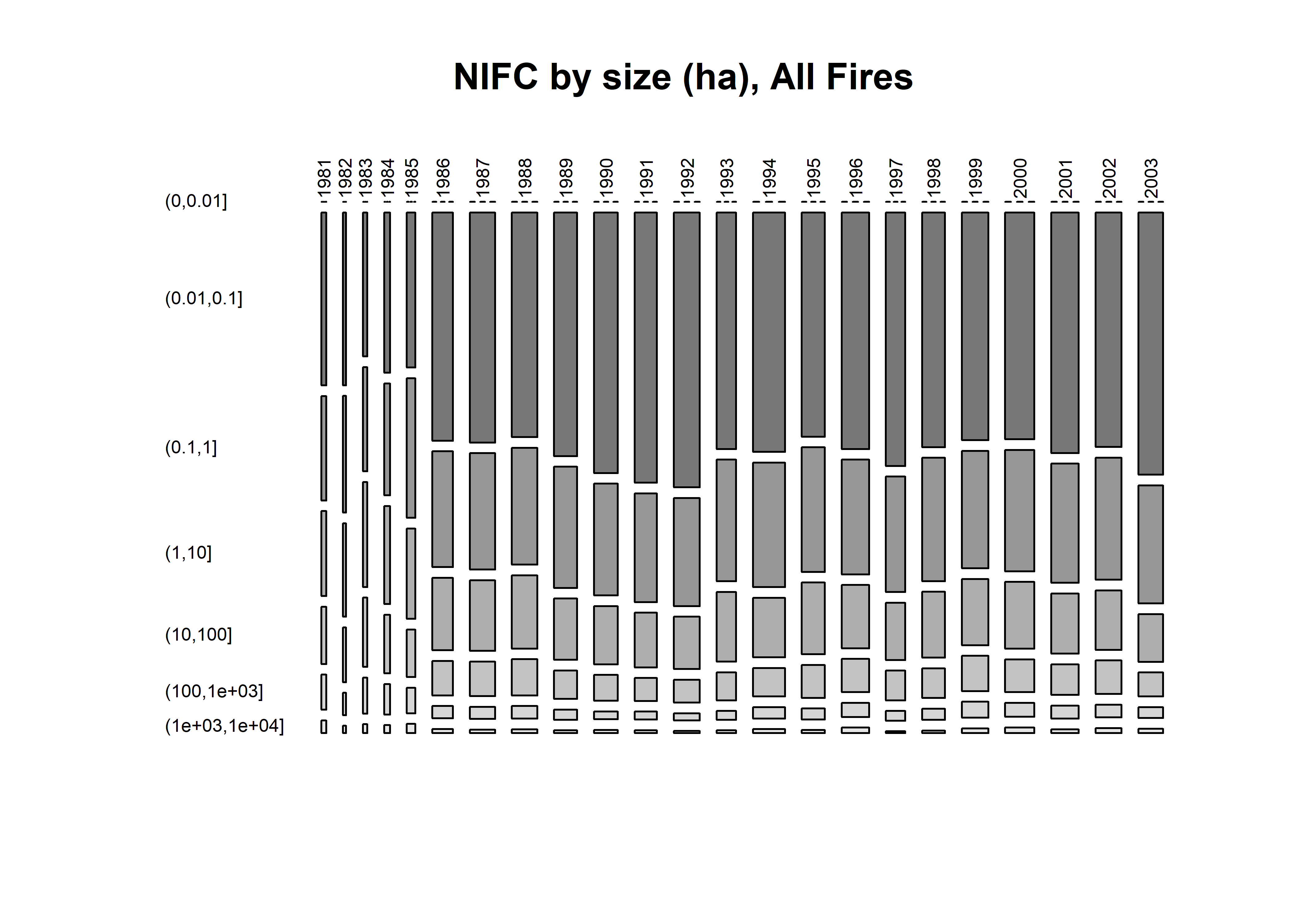
fwfod$sizeclass <- cut(fwfod$AREA,sizecuts)
table(fwfod$sizeclass)
##
## (0,0.01] (0.01,0.1] (0.1,1] (1,10] (10,100] (100,1e+03] (1e+03,1e+04]
## 2436 292483 146762 76340 36929 13957 4752fwfod.tablesize <- table(fwfod$startyear, fwfod$sizeclass)
mosaicplot(fwfod.tablesize, color=TRUE, cex.axis=0.6, las=2, main="FWFOD by size (ha), All Fires")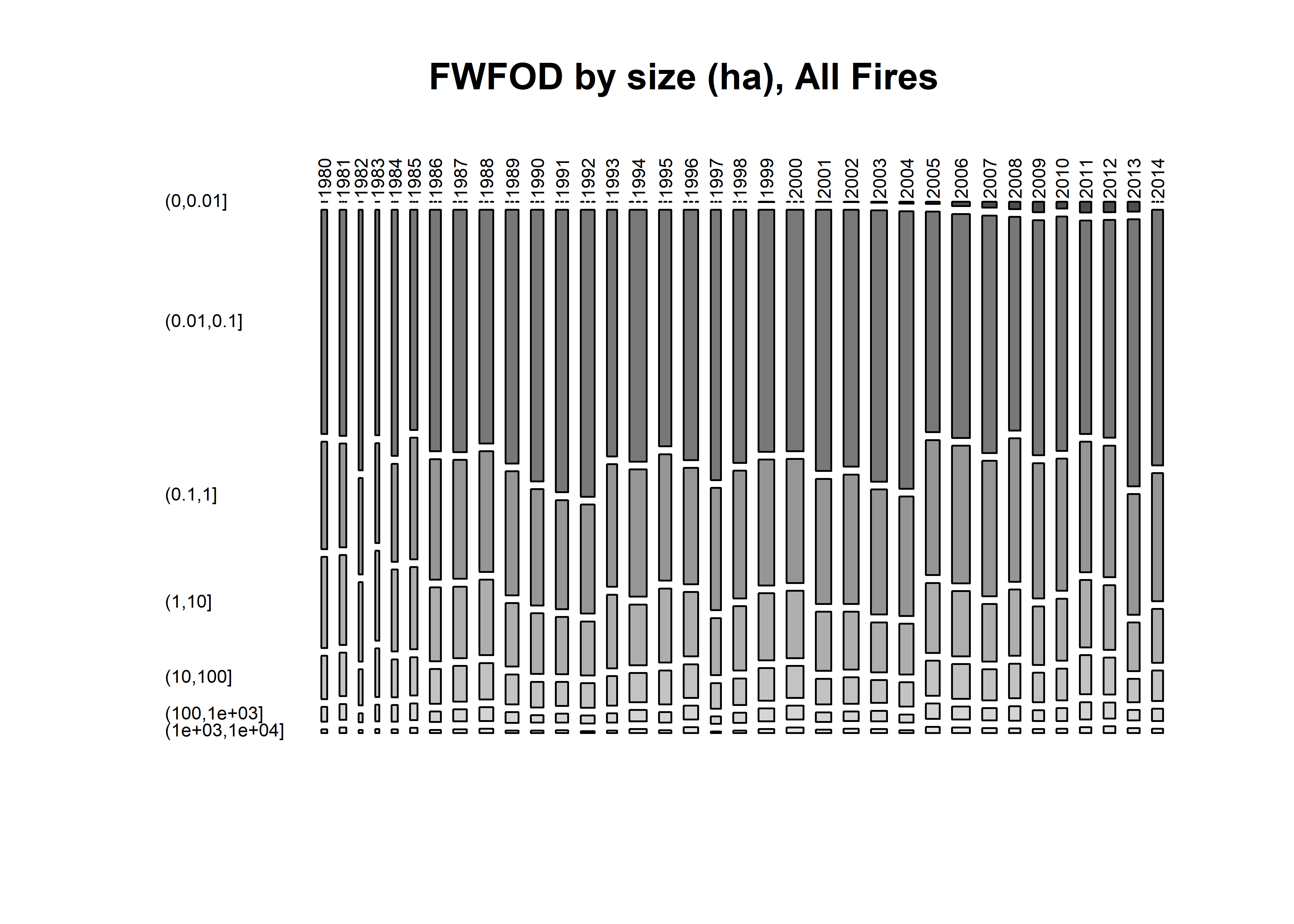
3.4 Fire areas by database
all_fpafod <- cbind(fpafod$FIRE_YEAR, fpafod$AREA_HA, "FPA-FOD")
all_nifc <- cbind(nifc$YEAR, nifc$AREA, "NIFC")
all_fwfod <- cbind(fwfod$startyear, fwfod$AREA, "FWFOD")
all_fires <-as.data.frame(rbind(all_fpafod,all_nifc,all_fwfod))
names(all_fires) <- c("Year","AreaHA", "db")
all_fires[,1] <- as.integer(as.character(all_fires[,1]))
all_fires[,2] <- as.numeric(as.character(all_fires[,2]))
all_fires <- na.omit(all_fires)

sizecuts <- c(0.0,0.00001,10,1000000) #
all_fires$sizeclass <- cut(all_fires$AreaHA,sizecuts)
table(all_fires$sizeclass)
##
## (0,1e-05] (1e-05,10] (10,1e+06]
## 1 2443878 237053all_tablesize <- table(all_fires$db, all_fires$sizeclass)
mosaicplot(all_tablesize, color=TRUE, cex.axis=0.6, las=2, main="All Fires -- Size (ha) by Database")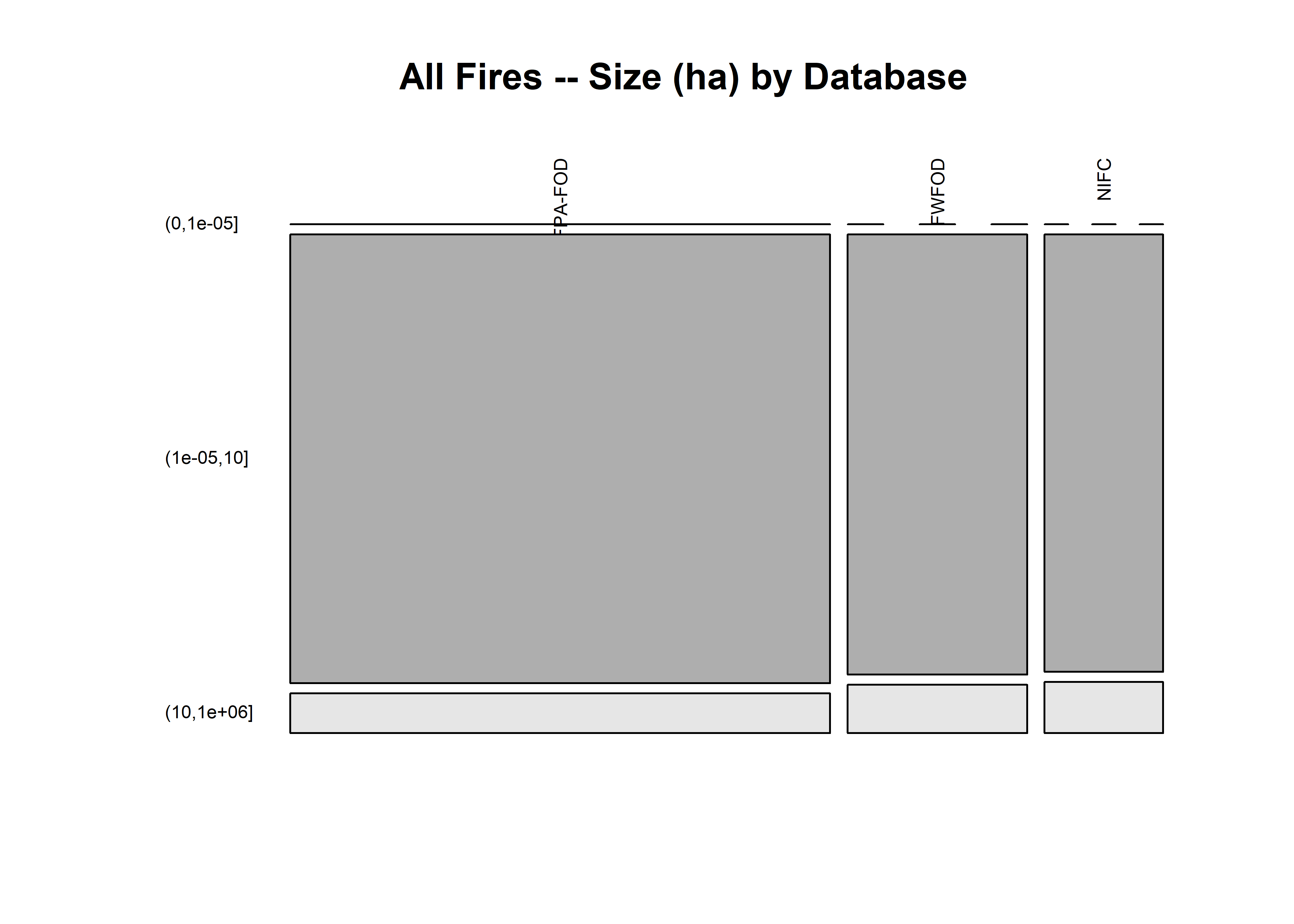
sizecuts <- c(0.0,0.01,0.1,1,10,100,1000,10000) # c(0.0,0.00001,10,1000000) #
all_fires$sizeclass <- cut(all_fires$AreaHA,sizecuts)
table(all_fires$sizeclass)
##
## (0,0.01] (0.01,0.1] (0.1,1] (1,10] (10,100] (100,1e+03] (1e+03,1e+04]
## 34179 1004633 897881 507186 176735 45115 12741all_tablesize <- table(all_fires$db, all_fires$sizeclass)
mosaicplot(all_tablesize, color=TRUE, cex.axis=0.6, las=2, main="All Fires -- Size (ha) by Database")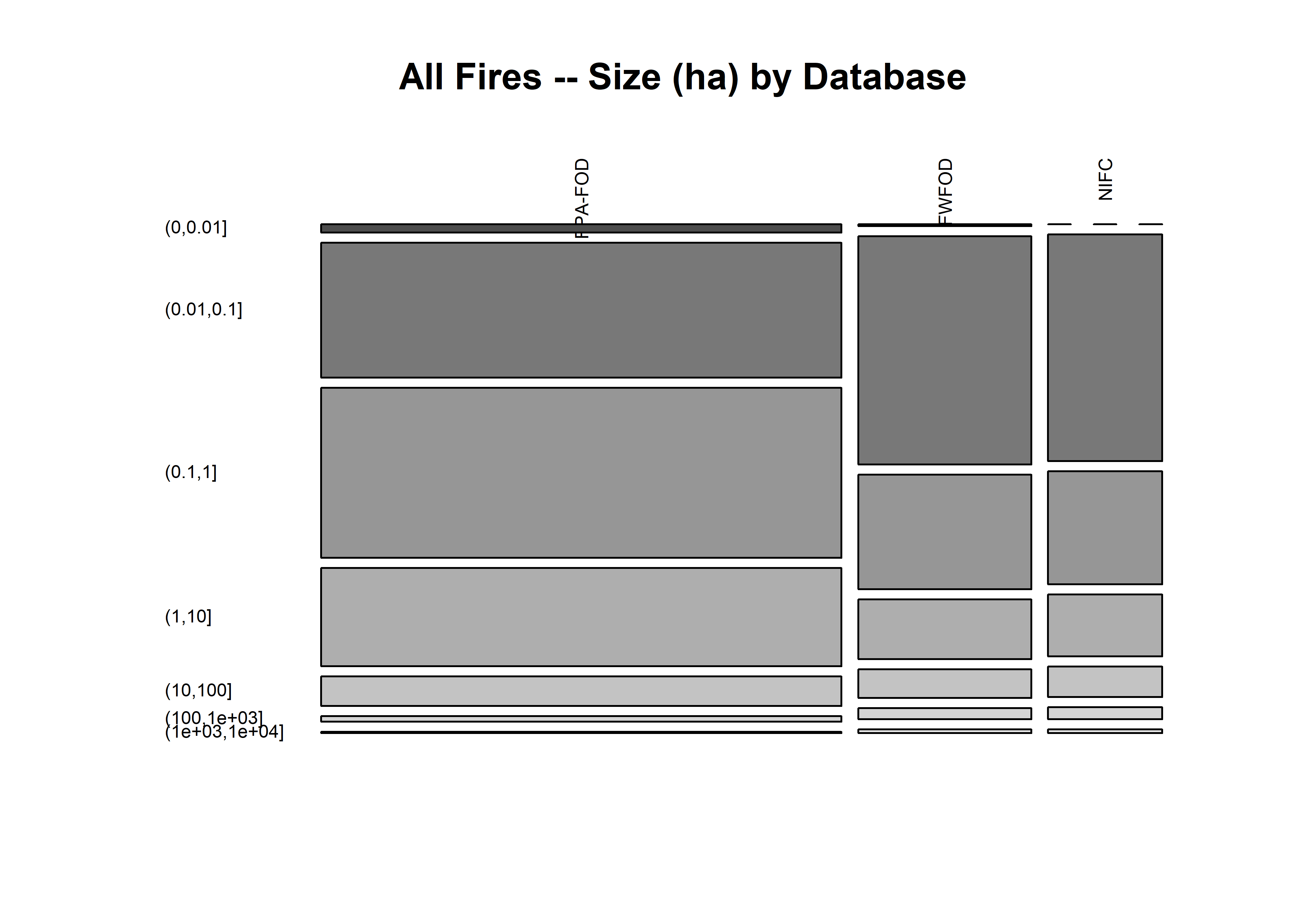
3.5 Fire frequency by month and year
fpafod.tablemon <- table(fpafod$FIRE_YEAR,
  fpafod$startmon)
mosaicplot(fpafod.tablemon, color=monthcolors, cex.axis=0.6, las=3, main="FPA-FOD, All Fires, All Agencies")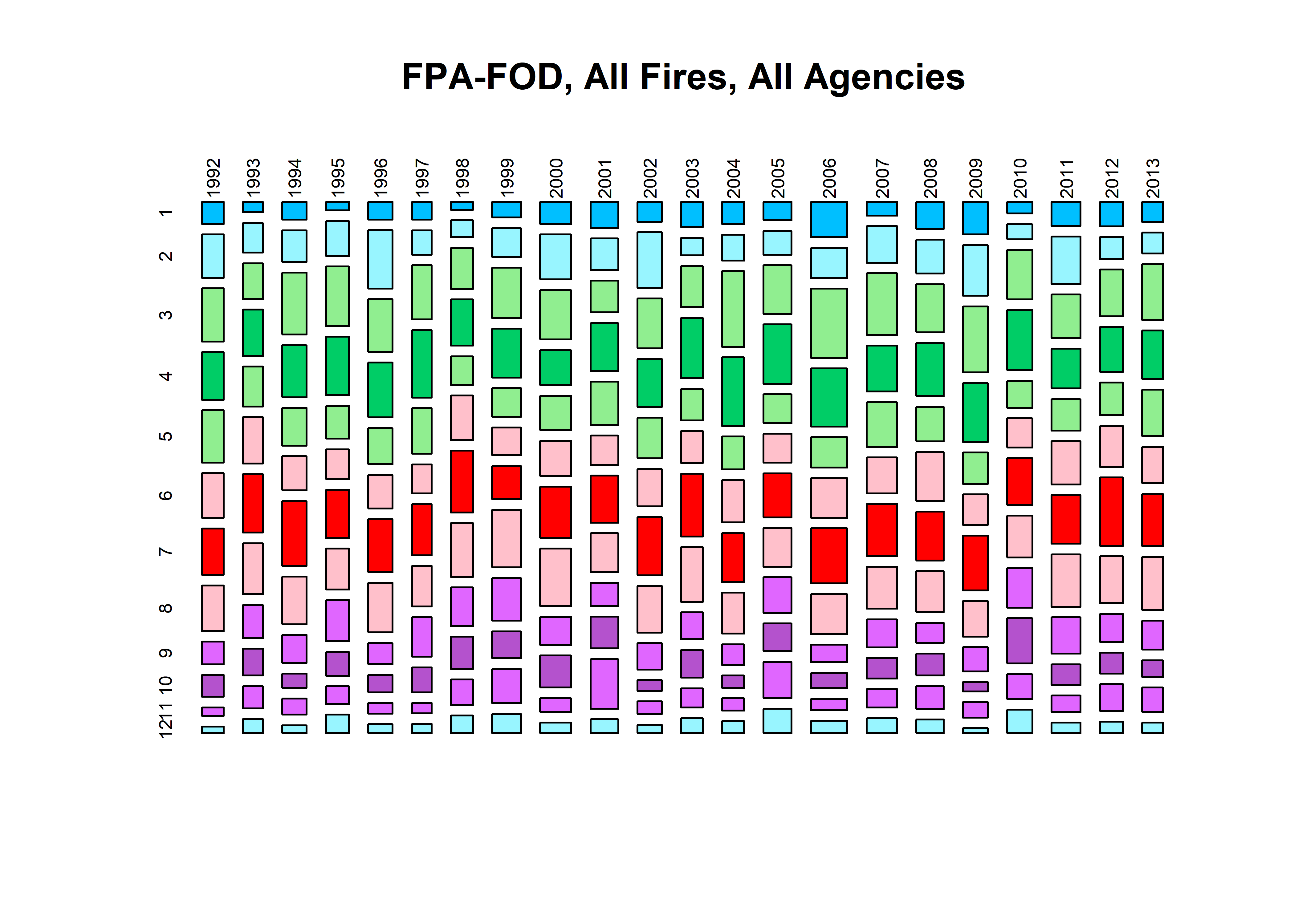
nifc.tablemon <- table(nifc$YEAR, nifc$startmon)
mosaicplot(nifc.tablemon, color=monthcolors, cex.axis=0.6, las=3, main="NIFC, All Fires, All Agencies")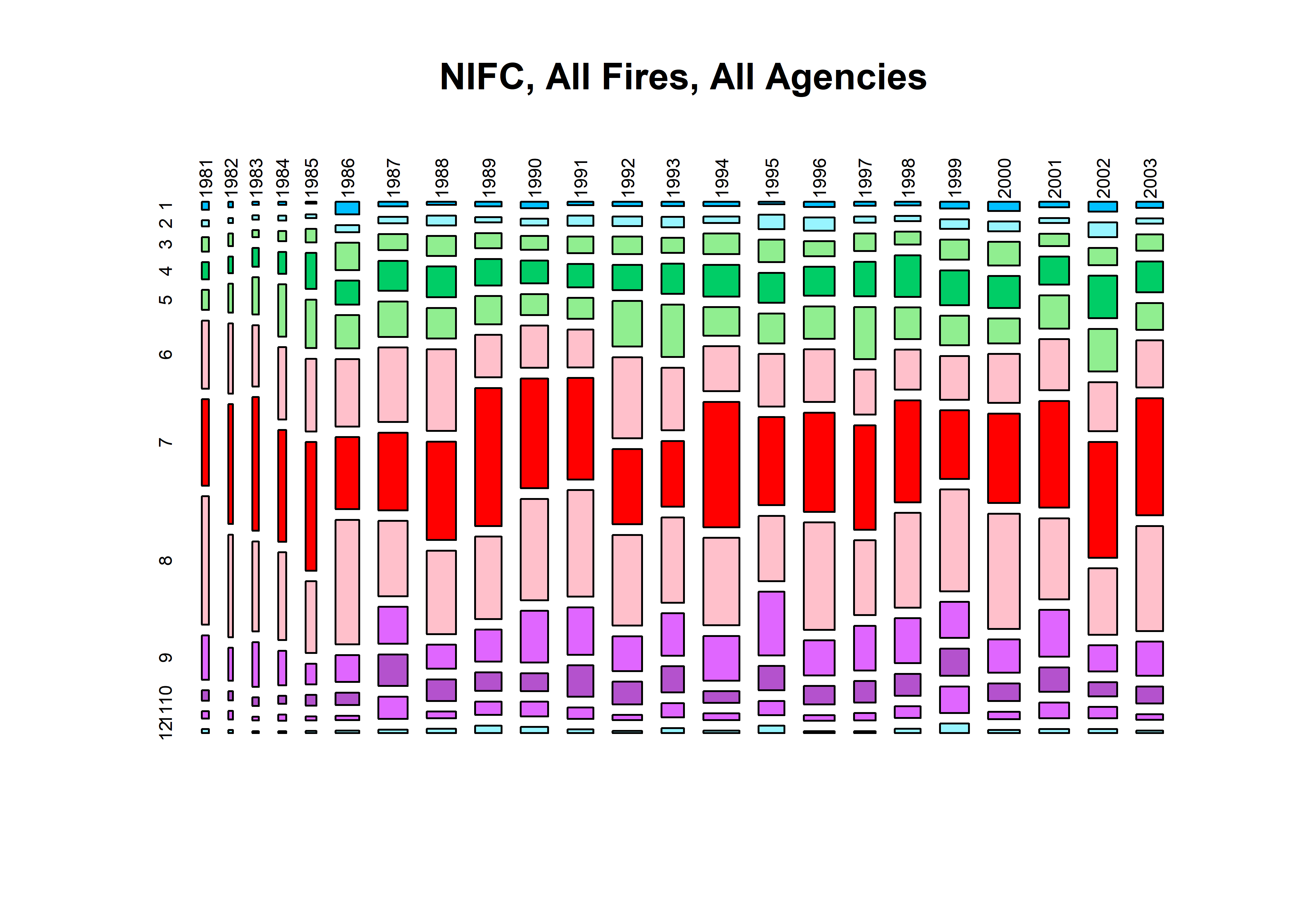
fwfod.tablemon <- table(fwfod$startyear, fwfod$startmon)
mosaicplot(fwfod.tablemon, color=monthcolors, cex.axis=0.6, las=3, main="FWFOD, All Fires, All Agencies")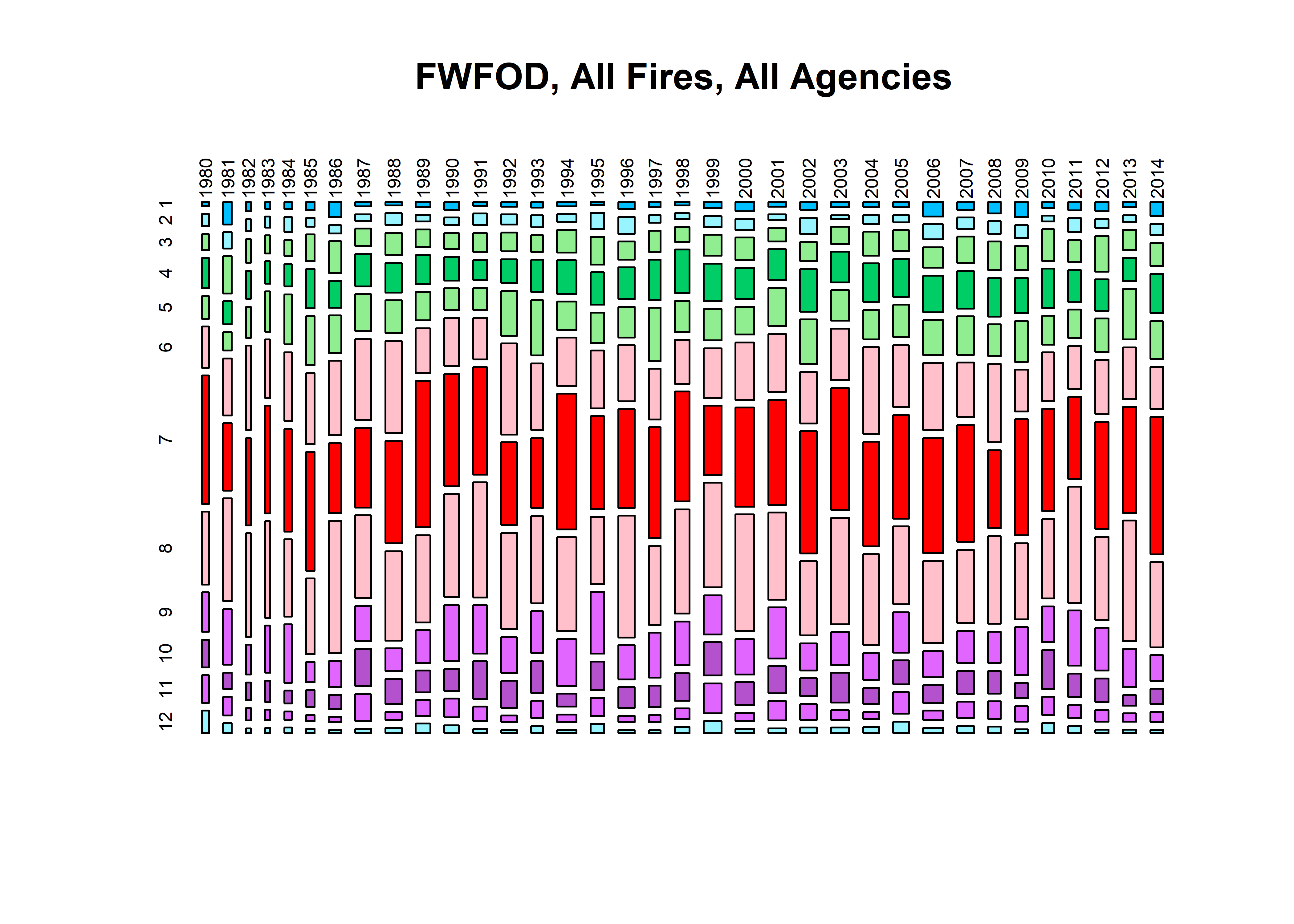
3.6 U.S. Forest Service
table(fpafod$FIRE_YEAR[fpafod$NWCG_REPORTING_AGENCY =="FS"])##
## 1992 1993 1994 1995 1996 1997 1998 1999 2000 2001 2002 2003 2004 2005 2006 2007 2008
## 11471 7731 14532 9231 11522 7913 9433 10994 11890 11018 9554 10727 8660 7661 10992 8960 7400
## 2009 2010 2011 2012 2013
## 7845 6951 7283 7518 7445table(nifc$YEAR[nifc$AGENCY_COD=="USFS"])##
## 1981 1982 1983 1984 1985 1986 1987 1988 1989 1990 1991 1992 1993 1994 1995 1996 1997
## 5 1 77 123 70 10604 13436 12718 11861 11875 10893 11649 7825 14751 9301 11580 7945
## 1998 1999 2000 2001 2002 2003
## 9471 11024 11983 11099 9538 10608table(fwfod$startyear[fwfod$ORGANIZATI=="FS"])##
## 1980 1981 1982 1983 1984 1985 1986 1987 1988 1989 1990 1991 1992 1993 1994 1995 1996
## 5860 6131 3601 3272 4722 4912 10713 13526 12832 11956 11985 10958 11755 7877 14793 9311 11595
## 1997 1998 1999 2000 2001 2002 2003 2004 2005 2006 2007 2008 2009 2010 2011 2012 2013
## 7956 9484 11092 11985 11135 9660 10785 8720 7766 11129 9003 7482 7815 6972 7422 7397 7245
## 2014
## 6733fpafod.tablemon <- table(fpafod$FIRE_YEAR[fpafod$NWCG_REPORTING_AGENCY == "FS" &
fpafod$STAT_CAUSE_CODE == 1], fpafod$startmon[fpafod$NWCG_REPORTING_AGENCY == "FS" &
fpafod$STAT_CAUSE_CODE == 1])
mosaicplot(fpafod.tablemon, color=monthcolors, cex.axis=0.6, las=3, main="FPA-FOD, All Fires, FS")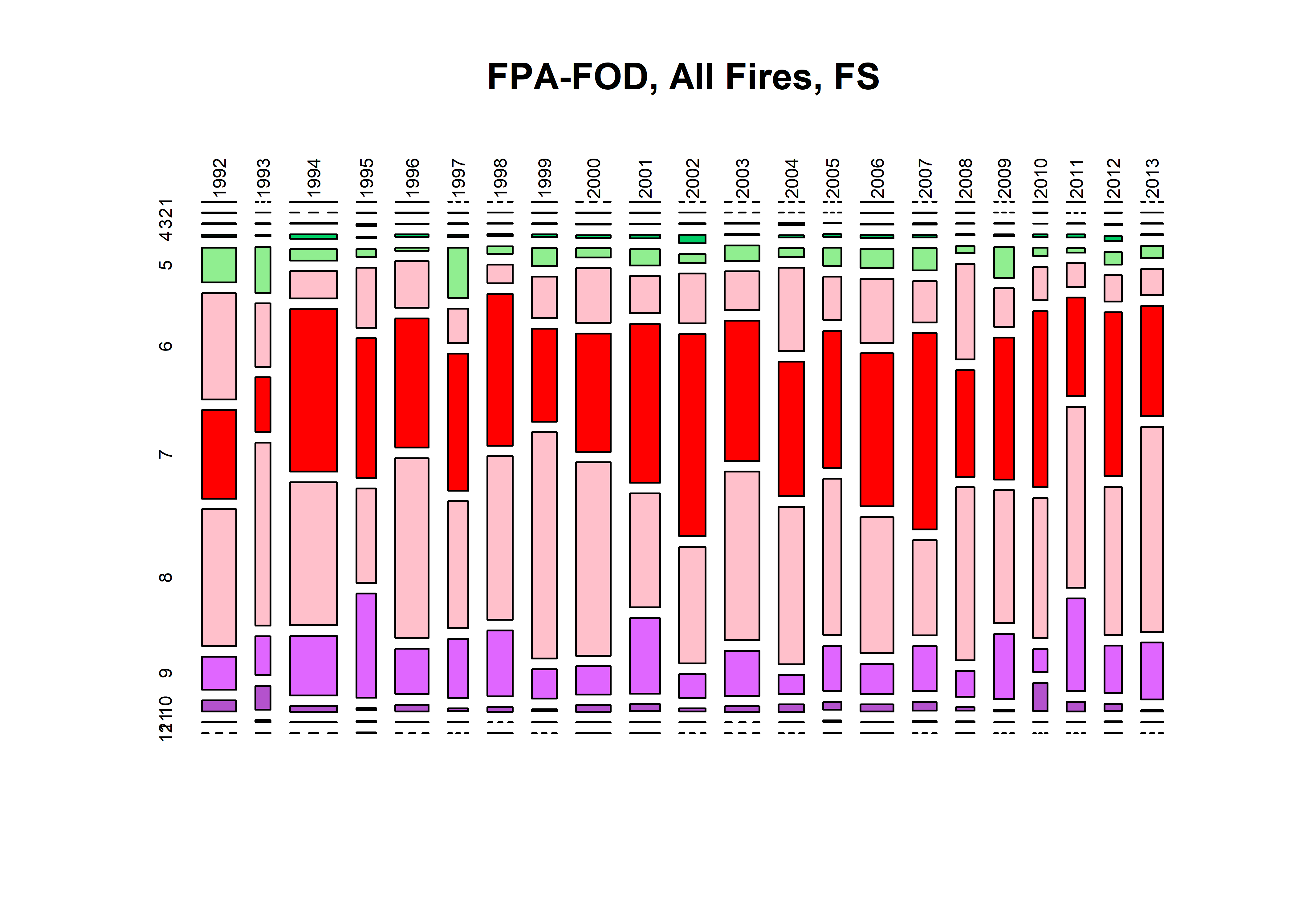
nifc.tablemon <- table(nifc$YEAR[nifc$AGENCY_COD== "USFS"],
  nifc$startmon[nifc$AGENCY_COD== "USFS"])
mosaicplot(nifc.tablemon, color=monthcolors, cex.axis=0.6, las=3, main="NIFC, All Fires, FS")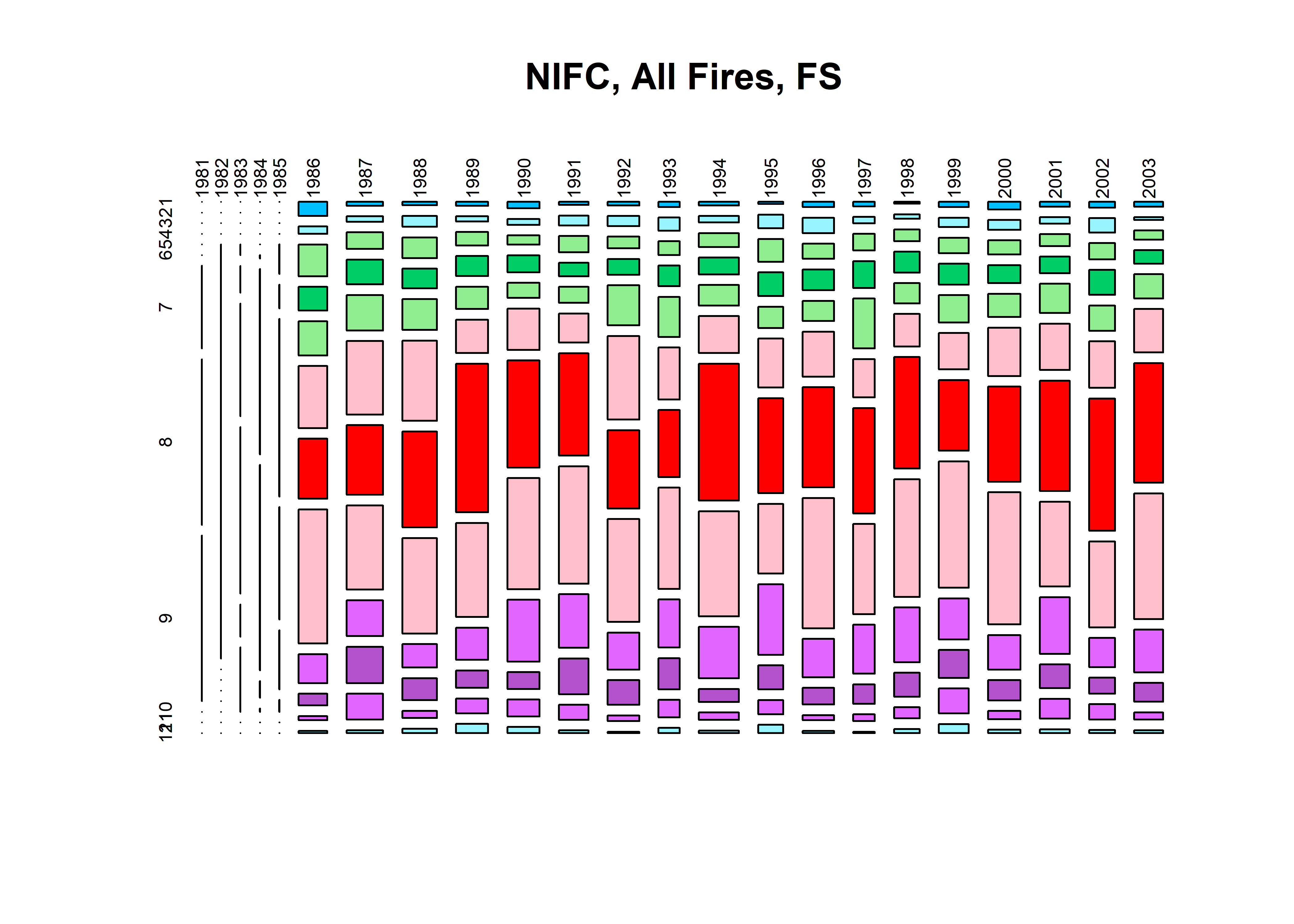
fwfod.tablemon <- table(fwfod$startyear[fwfod$ORGANIZATI== "FS"],
  fwfod$startmon[fwfod$ORGANIZATI== "FS"])
mosaicplot(fwfod.tablemon, color=monthcolors, cex.axis=0.6, las=3, main="NIFC, All Fires, FS")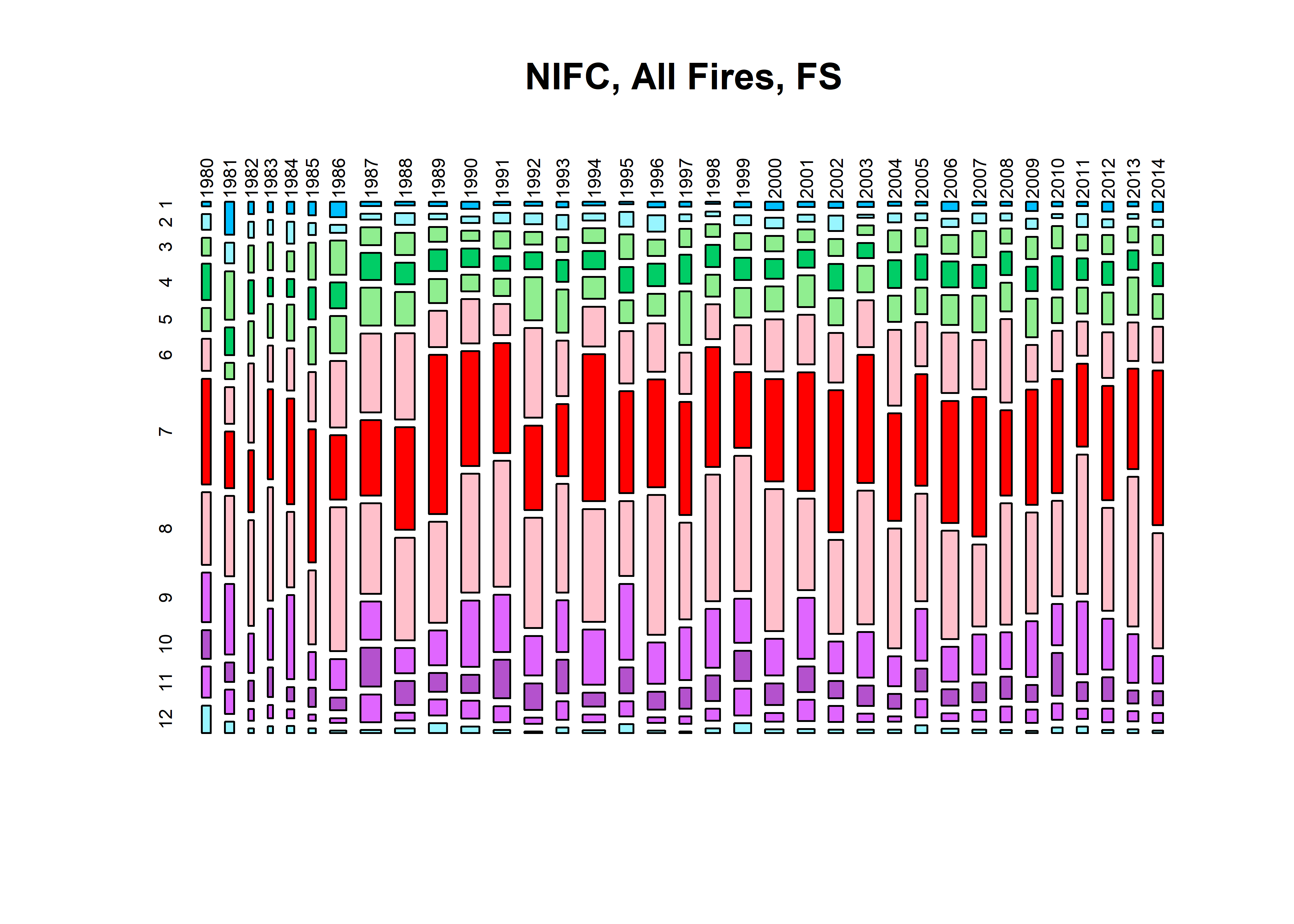
hist(nifc$YEAR, xlim=c(1980,2015), ylim=c(0,120000),
   breaks=seq(1979.5,2014.5,by=1), col="lightblue", border="blue", main="All Fires")
hist(fpafod$FIRE_YEAR, xlim=c(1980,2015), ylim=c(0,120000),
  breaks=seq(1979.5,2014.5,by=1), xlab="Year", col="pink", border="red", add=TRUE)
hist(fwfod$startyear, xlim=c(1980,2015), ylim=c(0,120000),
  breaks=seq(1979.5,2014.5,by=1), add=TRUE,  border="purple")
hist(nifc$YEAR, xlim=c(1980,2015), ylim=c(0,120000),
   breaks=seq(1979.5,2014.5,by=1), border="blue", add=TRUE)
legend("topleft", legend=c("FPA-FOD","NIFC","FWFOD"), lwd=2, col=c("red","blue","purple"))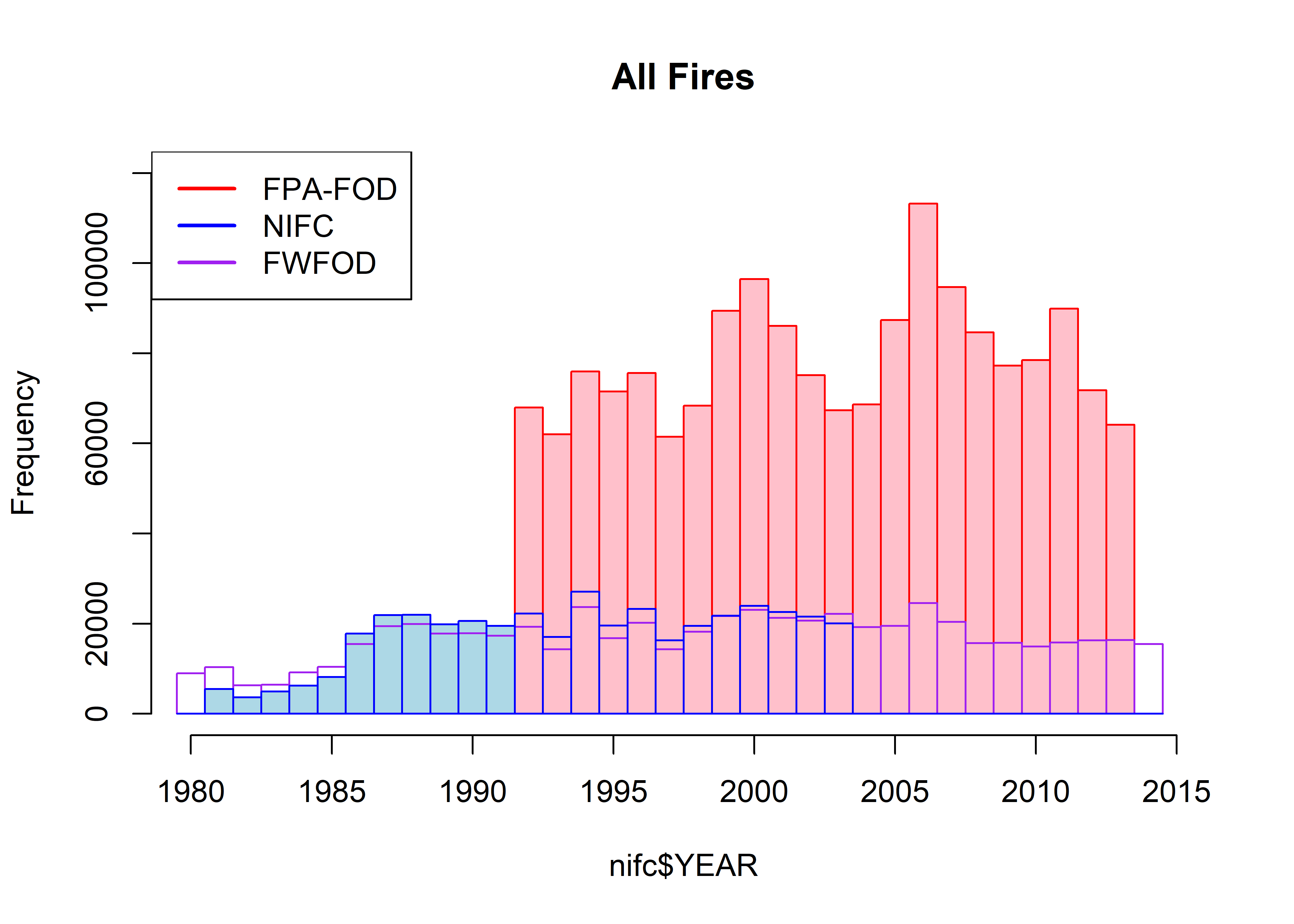
hist(nifc$YEAR[nifc$AGENCY_COD=="USFS"], xlim=c(1980,2015), ylim=c(0,120000),
   breaks=seq(1979.5,2014.5,by=1), col="lightblue", border="blue", main="All Fires, USFS")
hist(fpafod$FIRE_YEAR[fpafod$NWCG_REPORTING_AGENCY =="FS"],
  xlim=c(1980,2015), ylim=c(0,120000), breaks=seq(1979.5,2014.5,by=1), xlab="Year", col="pink", border="red",
  add=TRUE)
hist(fwfod$startyear[fwfod$ORGANIZATI=="FS"], xlim=c(1980,2015), ylim=c(0,120000),
  breaks=seq(1979.5,2014.5,by=1), add=TRUE, border="purple")
hist(nifc$YEAR[nifc$AGENCY_COD=="USFS"], xlim=c(1980,2015), ylim=c(0,120000),
   breaks=seq(1979.5,2014.5,by=1), border="blue", add=TRUE)
legend("topleft", legend=c("FPA-FOD","NIFC","FWFOD"), lwd=2, col=c("red","blue","purple"))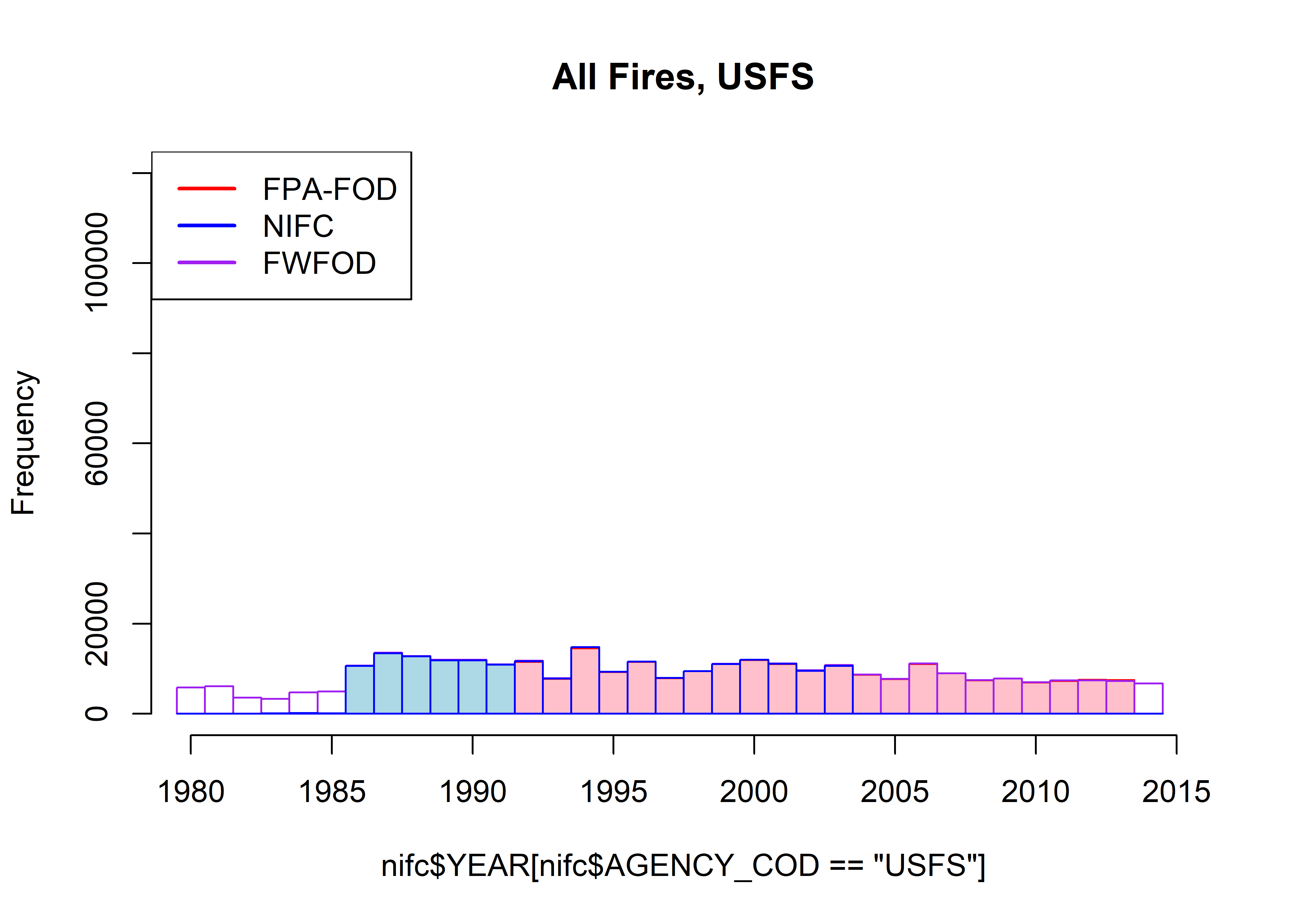
4 Compare FPA-FOD, FWFOD, and NIFC – Lightning/natural fires
Get lightning-started fires
fpafod_lt <- fpafod[fpafod$STAT_CAUSE_CODE == 1, ]
nifc_lt <- nifc[nifc$GENERAL_CA == 1, ]
fwfod_lt <- fwfod[fwfod$CAUSE == "Natural", ]
4.1 Maps
library(maps)
plot(fpafod_lt$LATITUDE ~ fpafod_lt$LONGITUDE, ylim=c(17,80), xlim=c(-180,-55), type="n",
  xlab="Longitude", ylab="Latitude", main="FPA-FOD -- Lightning Fires")
map("world", add=TRUE, lwd=2, col="gray")
points(fpafod_lt$LATITUDE ~ fpafod_lt$LONGITUDE, pch=16, cex=0.2, col="red")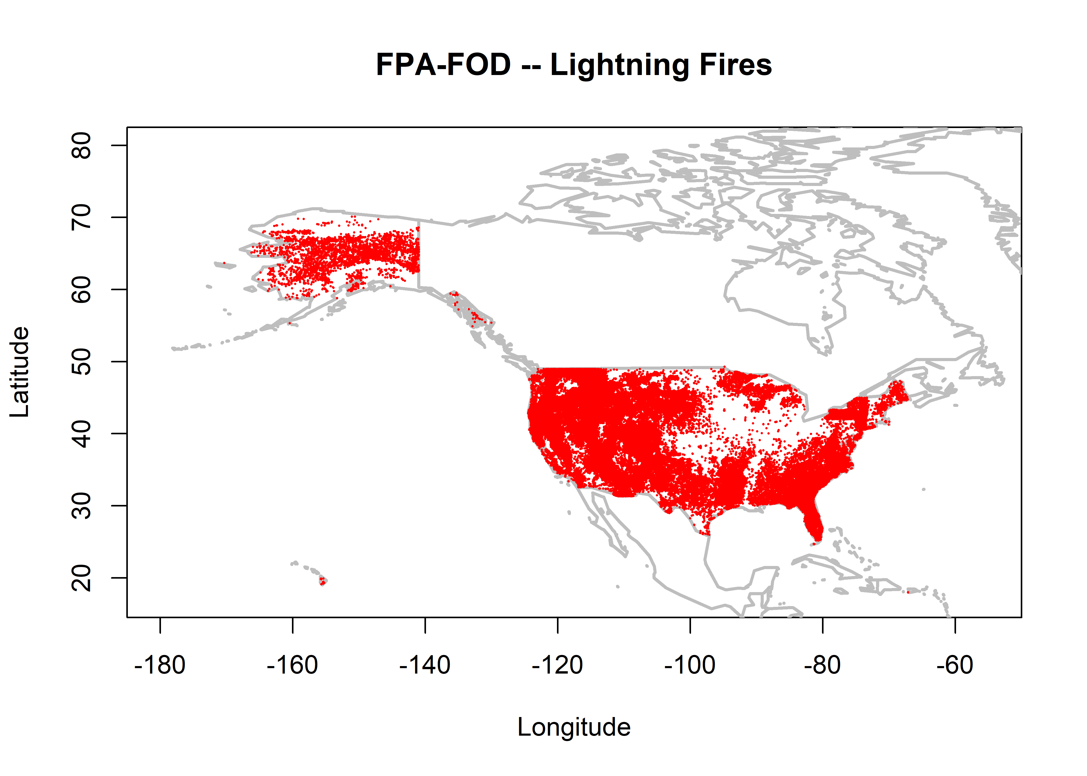
plot(nifc_lt$LATITUDE ~ nifc_lt$LONGITUDE, ylim=c(17,80), xlim=c(-180,-55), type="n",
  xlab="Longitude", ylab="Latitude", main="NIFC -- Lightning Fires")
map("world", add=TRUE, lwd=2, col="gray")
points(nifc_lt$LATITUDE ~ nifc_lt$LONGITUDE, pch=16, cex=0.2, col="red")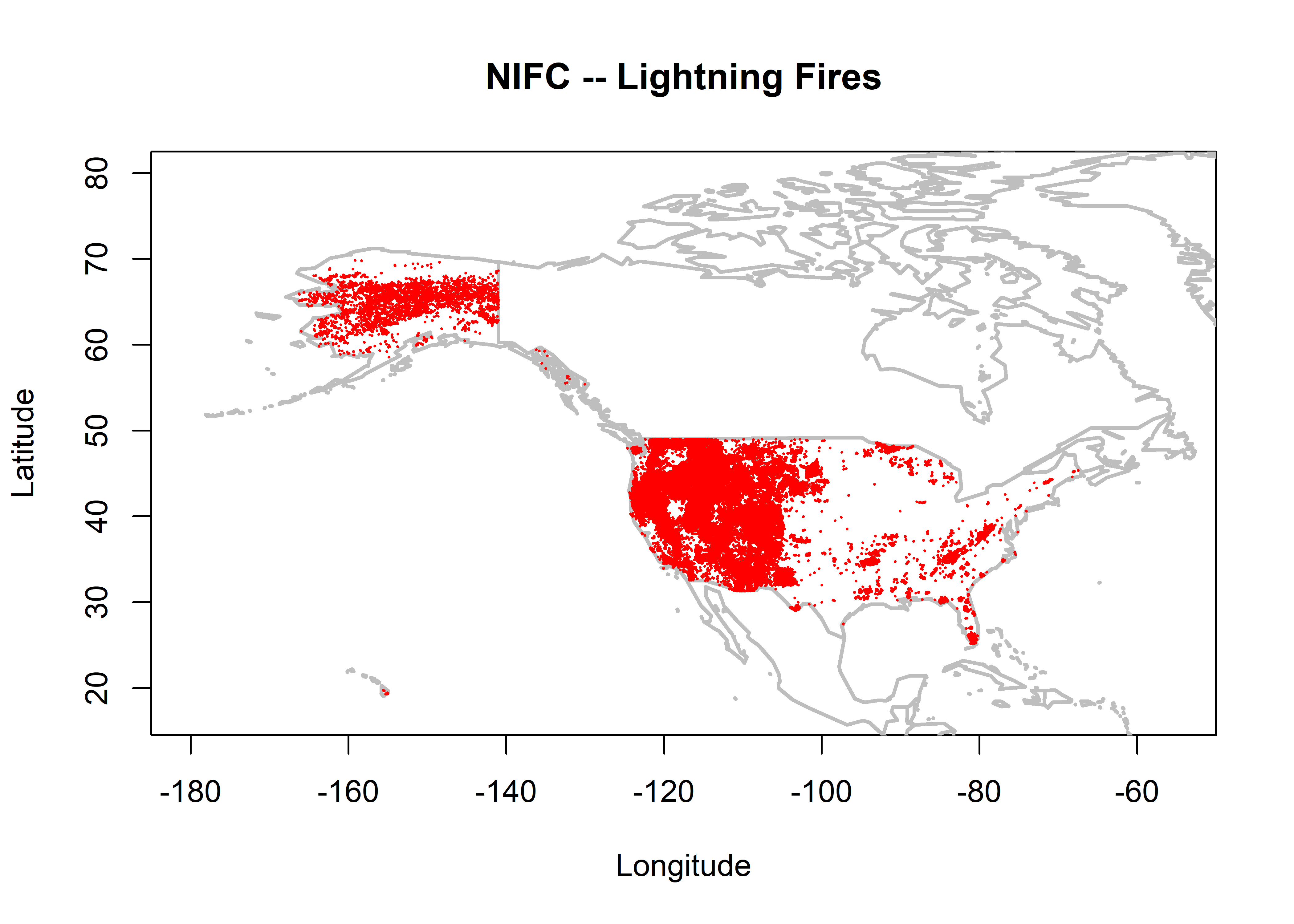
plot(fwfod_lt$DLATITUDE ~ fwfod_lt$DLONGITUDE, ylim=c(17,80), xlim=c(-180,-55), type="n",
  xlab="Longitude", ylab="Latitude", main="FWFOD -- Lightning Fires")
map("world", add=TRUE, lwd=2, col="gray")
points(fwfod_lt$DLATITUDE ~ fwfod_lt$DLONGITUDE, pch=16, cex=0.2, col="red")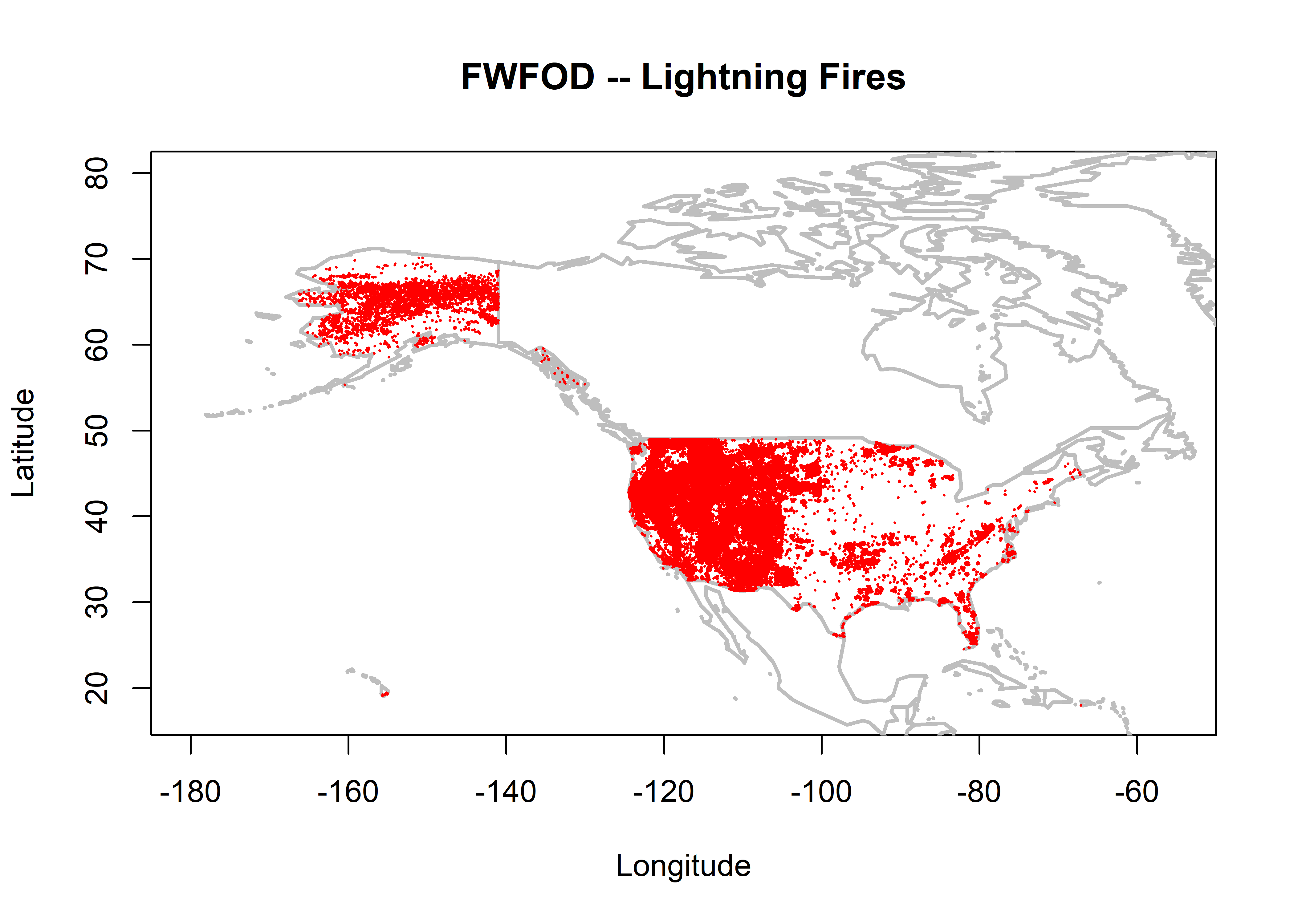
4.2 Time series – number and area
4.2.1 Total number of fires
Plot the fire count data.
fpafod_lt_num <- hist(fpafod_lt$FIRE_YEAR, breaks=seq(1979.5,2015.5, by=1), plot = FALSE)
nifc_lt_num <- hist(nifc_lt$YEAR, breaks=seq(1979.5,2015.5, by=1), plot = FALSE)
fwfod_lt_num <- hist(fwfod_lt$startyear, breaks=seq(1979.5,2015.5,by=1), plot = FALSE)

all_num_lt <- data.frame(fpafod_lt_num$mids, fpafod_lt_num$counts, nifc_lt_num$counts, fwfod_lt_num$counts)
all_num_lt[all_num_lt == 0] <- NA
names(all_num_lt) <- c("Year", "fpafod_lt_num", "nifc_lt_num", "fwfod_lt_num")
all_num_lt
## Year fpafod_lt_num nifc_lt_num fwfod_lt_num
## 1 1980 NA NA 3069
## 2 1981 NA 2443 3959
## 3 1982 NA 1452 2598
## 4 1983 NA 1953 2517
## 5 1984 NA 2553 4115
## 6 1985 NA 2980 4127
## 7 1986 NA 8620 7003
## 8 1987 NA 10167 8470
## 9 1988 NA 10216 9490
## 10 1989 NA 9872 8653
## 11 1990 NA 10897 8332
## 12 1991 NA 8857 9200
## 13 1992 12240 10540 10207
## 14 1993 7545 5193 4925
## 15 1994 16212 14035 9624
## 16 1995 8078 6424 7321
## 17 1996 12643 10900 9989
## 18 1997 8456 6612 6185
## 19 1998 10893 7589 7280
## 20 1999 11810 8260 7985
## 21 2000 16559 12028 11248
## 22 2001 13842 10648 9632
## 23 2002 12480 9138 8739
## 24 2003 13849 11281 11392
## 25 2004 11732 NA 9243
## 26 2005 11104 NA 7209
## 27 2006 16958 NA 11162
## 28 2007 12719 NA 8055
## 29 2008 9914 NA 5840
## 30 2009 10492 NA 6656
## 31 2010 8980 NA 5358
## 32 2011 12539 NA 6391
## 33 2012 11130 NA 6305
## 34 2013 10136 NA 7961
## 35 2014 NA NA 6367
## 36 2015 NA NA NATime series plots of the numbers of fires:
plot(all_num_lt$fpafod_lt_num ~ all_num_lt$Year, type="o", col="red", pch=16, xlim=c(1980,2015),
     ylim=c(0,25000),xlab="Year", ylab="Total Number of Lighting/Natural Fires",
     main="Total Number of Fires (U.S. LIghtning/Natural)", lwd=2)
lines(all_num_lt$nifc_lt_num ~ all_num_lt$Year, type="o", col="blue", pch=16, lwd=2)
lines(all_num_lt$fwfod_lt_num ~ all_num_lt$Year, type="o", col="purple", pch=16, lwd=2)
legend("topleft", legend=c("FPA-FOD","NIFC","FWFOD"), lwd=2, col=c("red","blue","purple"))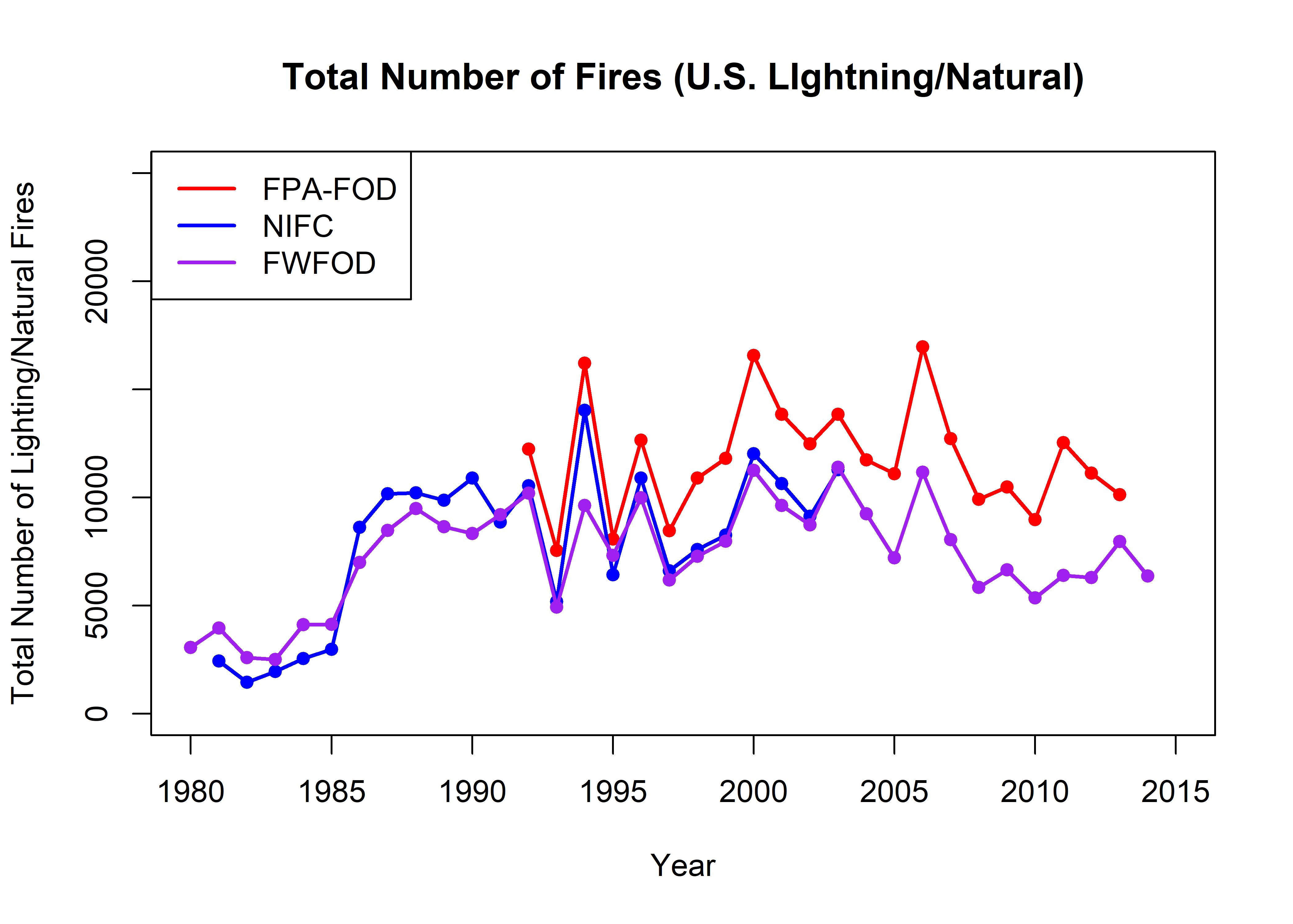
Scatter plots that compare the three different data sets:
oldpar <- par(mfrow=c(1,3))
plot(all_num_lt$fpafod_lt_num, all_num_lt$nifc_lt_num, xlim=c(0,25000), ylim=c(0,25000), pch=16,
     xlab="FPA-FOD", ylab="NIFC"); abline(0,1); abline(0,1)
plot(all_num_lt$fpafod_lt_num, all_num_lt$fwfod_lt_num, xlim=c(0,25000), ylim=c(0,25000), pch=16,
     xlab="FPA-FOD", ylab="FWFOD",
     main="Total Number of Fires (U.S. LIghtning/Natural)"); abline(0,1); abline(0,1)
plot(all_num_lt$fwfod_lt_num, all_num_lt$nifc_lt_num, xlim=c(0,25000), ylim=c(0,25000), pch=16,
     xlab="FWFOD", ylab="NIFC"); abline(0,1); abline(0,1)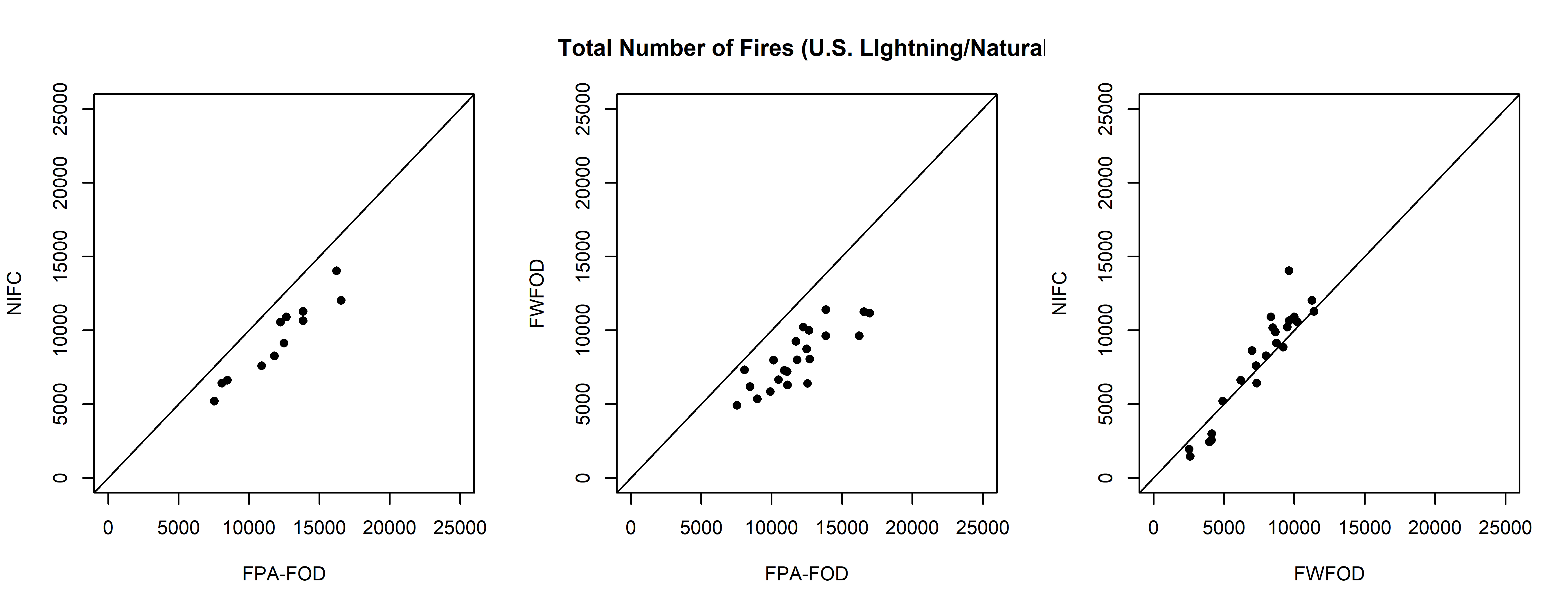
par(oldpar)4.2.2 Total area burned
Get time series of total area burned.
all_totalarea_lt <- data.frame(matrix(nrow = 36, ncol = 4))
names(all_totalarea_lt) <- c("Year", "fpafod_lt_totalarea", "nifc_lt_totalarea",
      "fwfod_lt_totalarea")
all_totalarea_lt["Year"] <- seq(1980, 2015, by=1)

fpafod_lt_total_by_year <- tapply(fpafod_lt$AREA_HA, fpafod_lt$FIRE_YEAR, sum)
fpafod_lt_year <- as.numeric(unlist(dimnames(fpafod_lt_total_by_year)))
fpafod_lt_total_by_year <- as.numeric(fpafod_lt_total_by_year)
all_totalarea_lt$fpafod_lt_totalarea[fpafod_lt_year-1980+1] <- fpafod_lt_total_by_year

fwfod_lt_total_by_year <- tapply(fwfod_lt$AREA, fwfod_lt$startyear, sum)
fwfod_lt_year <- as.numeric(unlist(dimnames(fwfod_lt_total_by_year)))
fwfod_lt_total_by_year <- as.numeric(fwfod_lt_total_by_year)
all_totalarea_lt$fwfod_lt_totalarea[fwfod_lt_year-1980+1] <- fwfod_lt_total_by_year

nifc_lt_size_year <- na.omit(cbind(nifc_lt$AREA,nifc_lt$YEAR))
nifc_lt_total_by_year <- tapply(nifc_lt_size_year[,1],nifc_lt_size_year[,2], sum)
nifc_lt_year <- as.numeric(unlist(dimnames(nifc_lt_total_by_year)))
nifc_lt_total_by_year <- as.numeric(nifc_lt_total_by_year)
all_totalarea_lt$nifc_lt_totalarea[nifc_lt_year-1980+1] <- nifc_lt_total_by_year

all_totalarea_lt
## Year fpafod_lt_totalarea nifc_lt_totalarea fwfod_lt_totalarea
## 1 1980 NA NA 126502.29
## 2 1981 NA 390658.00 443102.32
## 3 1982 NA 74543.61 75344.48
## 4 1983 NA 337226.87 146670.14
## 5 1984 NA 370424.07 298361.59
## 6 1985 NA 605549.10 550408.37
## 7 1986 NA 701069.33 409890.46
## 8 1987 NA 716904.97 499343.80
## 9 1988 NA 1922016.82 2582652.63
## 10 1989 NA 360364.38 271143.18
## 11 1990 NA 1475366.70 1267875.33
## 12 1991 NA 764601.51 990557.17
## 13 1992 407584.4 463106.47 347785.43
## 14 1993 450158.4 424814.27 571797.06
## 15 1994 968704.7 1014253.96 796911.11
## 16 1995 336450.7 298895.62 293495.28
## 17 1996 1315241.4 1287338.70 1231879.24
## 18 1997 897751.6 809226.56 895369.23
## 19 1998 338368.9 183561.24 215309.26
## 20 1999 1483206.9 1268250.84 1194435.67
## 21 2000 1981239.1 2048149.64 1999220.02
## 22 2001 791011.1 679550.88 486658.99
## 23 2002 1619161.5 1885939.51 1891291.08
## 24 2003 984487.1 999180.22 1113437.61
## 25 2004 2905897.9 NA 3724948.64
## 26 2005 3077578.0 NA 4667100.14
## 27 2006 2249413.5 NA 2015165.83
## 28 2007 2417510.5 NA 2061759.56
## 29 2008 905480.5 NA 915739.31
## 30 2009 1593883.2 NA 1949517.35
## 31 2010 821844.7 NA 866470.95
## 32 2011 1541435.7 NA 943460.88
## 33 2012 2785734.5 NA 2071088.86
## 34 2013 1214911.1 NA 1314080.18
## 35 2014 NA NA 921689.52
## 36 2015 NA NA NAplot(all_totalarea_lt$fpafod_lt_totalarea ~ all_totalarea_lt$Year, type="o", col="red", pch=16, lwd=2, xlim=c(1980,2015), ylim=c(0,6000000),xlab="Year", ylab="Total Area Burned",
main="Total Area Burned (ha) (U.S. Lightning/Natural)")
points(all_totalarea_lt$fwfod_lt_totalarea ~ all_totalarea_lt$Year, type="o", col="purple", pch=16,
lwd=2)
points(all_totalarea_lt$nifc_lt_totalarea ~ all_totalarea_lt$Year, type="o", col="blue", pch=16,
lwd=2)
legend("topleft", legend=c("FPA-FOD","NIFC","FWFOD"), lwd=2, col=c("red","blue","purple"))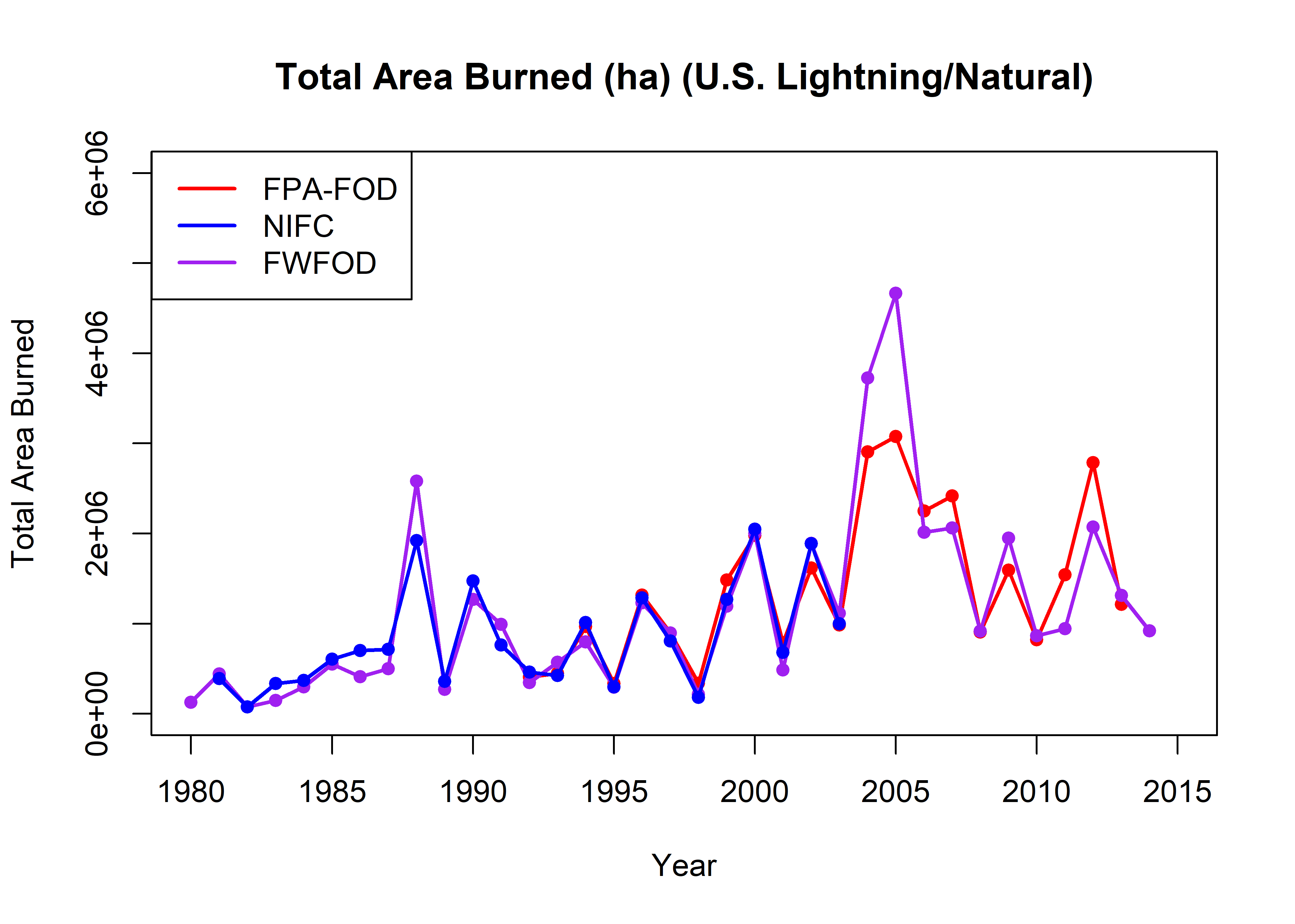
Scatter plots of the total areas burned in each data set:
oldpar <- par(mfrow=c(1,3))
plot(all_totalarea_lt$fpafod_lt_totalarea, all_totalarea_lt$nifc_lt_totalarea, xlim=c(0,6000000),
     ylim=c(0,6000000), pch=16, xlab="FPA-FOD", ylab="nifc_lt"); abline(0,1)
plot(all_totalarea_lt$fpafod_lt_totalarea, all_totalarea_lt$fwfod_lt_totalarea, xlim=c(0,6000000),
     ylim=c(0,6000000), pch=16, xlab="FPA-FOD", ylab="fwfod_lt",
     main="Total Area Burned (ha) (U.S. Lightning)"); abline(0,1)
plot(all_totalarea_lt$fwfod_lt_totalarea, all_totalarea_lt$nifc_lt_totalarea, xlim=c(0,6000000),
     ylim=c(0,6000000), pch=16, xlab="FWFOD", ylab="NIFC"); abline(0,1)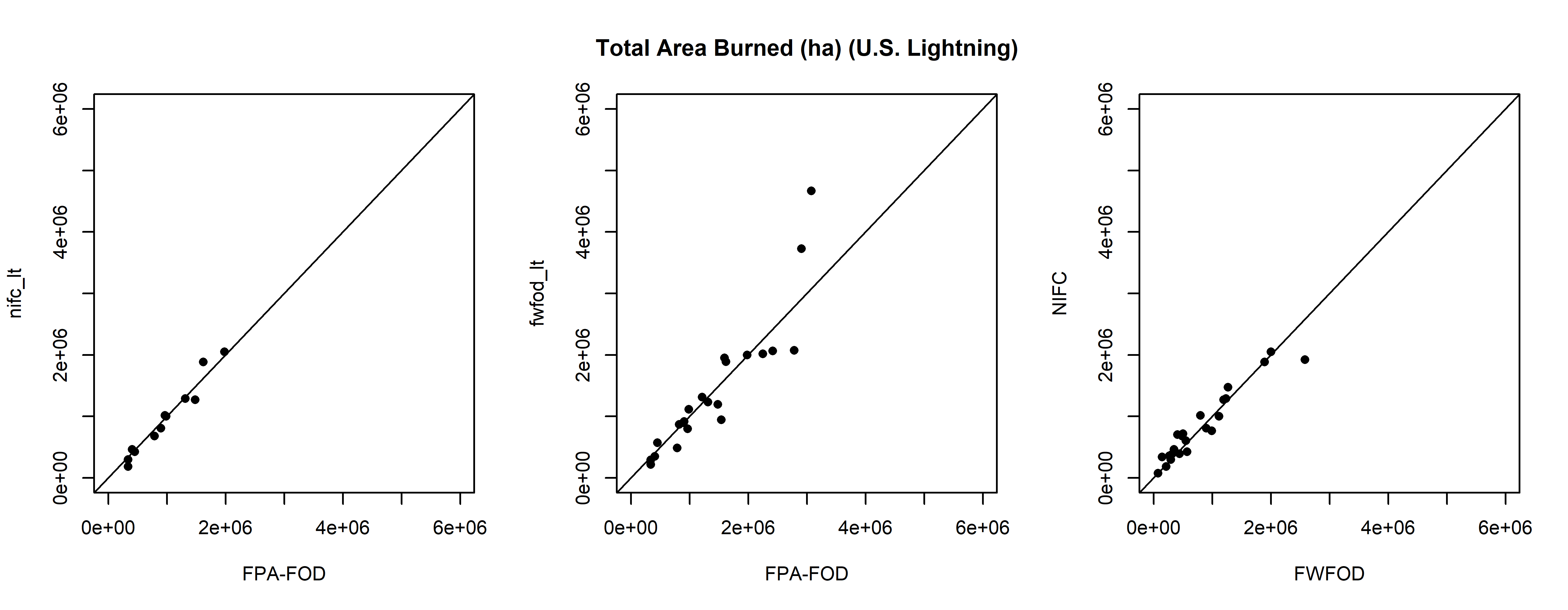
par(oldpar)4.2.3 Mean area burned
all_meanarea_lt <- data.frame(matrix(nrow = 36, ncol = 4))
names(all_meanarea_lt) <- c("Year", "fpafod_lt_meanarea", "nifc_lt_meanarea", "fwfod_lt_meanarea")
all_meanarea_lt["Year"] <- seq(1980, 2015, by=1)

fpafod_lt_mean_by_year <- tapply(fpafod_lt$AREA_HA, fpafod_lt$FIRE_YEAR, mean)
fpafod_lt_year <- as.numeric(unlist(dimnames(fpafod_lt_mean_by_year)))
fpafod_lt_mean_by_year <- as.numeric(fpafod_lt_mean_by_year)
all_meanarea_lt$fpafod_lt_meanarea[fpafod_lt_year-1980+1] <- fpafod_lt_mean_by_year

fwfod_lt_mean_by_year <- tapply(fwfod_lt$AREA, fwfod_lt$startyear, mean)
fwfod_lt_year <- as.numeric(unlist(dimnames(fwfod_lt_mean_by_year)))
fwfod_lt_mean_by_year <- as.numeric(fwfod_lt_mean_by_year)
all_meanarea_lt$fwfod_lt_meanarea[fwfod_lt_year-1980+1] <- fwfod_lt_mean_by_year

nifc_lt_size_year <- na.omit(cbind(nifc_lt$AREA,nifc_lt$YEAR))
nifc_lt_mean_by_year <- tapply(nifc_lt_size_year[,1],nifc_lt_size_year[,2], mean)
nifc_lt_year <- as.numeric(unlist(dimnames(nifc_lt_mean_by_year)))
nifc_lt_mean_by_year <- as.numeric(nifc_lt_mean_by_year)
all_meanarea_lt$nifc_lt_meanarea[nifc_lt_year-1980+1] <- nifc_lt_mean_by_year

all_meanarea_lt
## Year fpafod_lt_meanarea nifc_lt_meanarea fwfod_lt_meanarea
## 1 1980 NA NA 41.21939
## 2 1981 NA 159.90913 111.92279
## 3 1982 NA 51.33857 29.00095
## 4 1983 NA 172.67121 58.27181
## 5 1984 NA 145.09364 72.50585
## 6 1985 NA 203.20440 133.36767
## 7 1986 NA 81.33055 58.53070
## 8 1987 NA 70.51293 58.95440
## 9 1988 NA 188.13790 272.14464
## 10 1989 NA 36.50369 31.33516
## 11 1990 NA 135.39201 152.16939
## 12 1991 NA 86.32737 107.66926
## 13 1992 33.29938 43.93800 34.07323
## 14 1993 59.66315 81.80517 116.10093
## 15 1994 59.75232 72.26605 82.80456
## 16 1995 41.65025 46.52796 40.08951
## 17 1996 104.02922 118.10447 123.32358
## 18 1997 106.16740 122.38756 144.76463
## 19 1998 31.06297 24.18780 29.57545
## 20 1999 125.58907 153.54126 149.58493
## 21 2000 119.64727 170.28181 177.74004
## 22 2001 57.14572 63.81958 50.52523
## 23 2002 129.74051 206.38428 216.41962
## 24 2003 71.08723 88.57195 97.73855
## 25 2004 247.68990 NA 403.00212
## 26 2005 277.15940 NA 647.39910
## 27 2006 132.64616 NA 180.53806
## 28 2007 190.07080 NA 255.96022
## 29 2008 91.33352 NA 156.80468
## 30 2009 151.91414 NA 292.89624
## 31 2010 91.51946 NA 161.71537
## 32 2011 122.93131 NA 147.62336
## 33 2012 250.29061 NA 328.48356
## 34 2013 119.86100 NA 165.06471
## 35 2014 NA NA 144.76041
## 36 2015 NA NA NAplot(fpafod_lt_mean_by_year ~ fpafod_lt_year, type="o", col="red", pch=16, lwd=2, xlim=c(1980,2015),
ylim=c(0,800), xlab="Year", ylab="Mean Area Burned",
main="Mean Area Burned (ha) (U.S. Lightning/Natural)")
points(fwfod_lt_mean_by_year ~ fwfod_lt_year, type="o", col="purple", pch=16, lwd=2)
points(nifc_lt_mean_by_year ~ nifc_lt_year, type="o", col="blue", pch=16, lwd=2)
legend("topleft", legend=c("FPA-FOD","NIFC","FWFOD"), lwd=2, col=c("red","blue","purple"))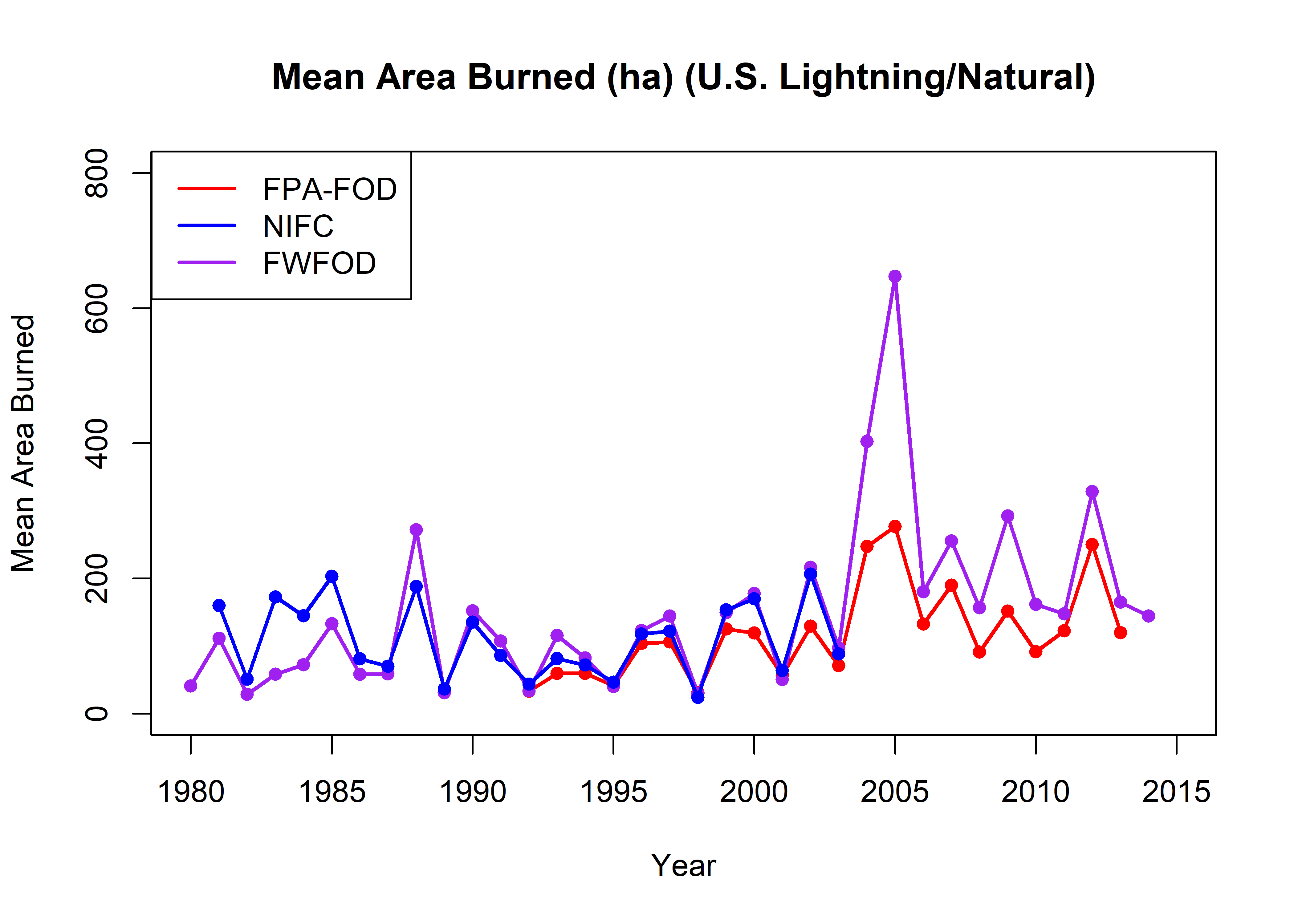
Scatter plots of the mean areas burned in each data set:
oldpar <- par(mfrow=c(1,3))
plot(all_meanarea_lt$fpafod_lt_meanarea, all_meanarea_lt$nifc_lt_meanarea, xlim=c(0,300),
     ylim=c(0,800), pch=16, xlab="FPA-FOD", ylab="NIFC"); abline(0,1)
plot(all_meanarea_lt$fpafod_lt_meanarea, all_meanarea_lt$fwfod_lt_meanarea, xlim=c(0,300),
     ylim=c(0,800), pch=16, xlab="FPA-FOD", ylab="FWFOD",
     main="Mean Area Burned (ha) (U.S. All)"); abline(0,1)
plot(all_meanarea_lt$fwfod_lt_meanarea, all_meanarea_lt$nifc_lt_meanarea, xlim=c(0,300),
     ylim=c(0,800 ), pch=16, xlab="FWFOD", ylab="NIFC"); abline(0,1)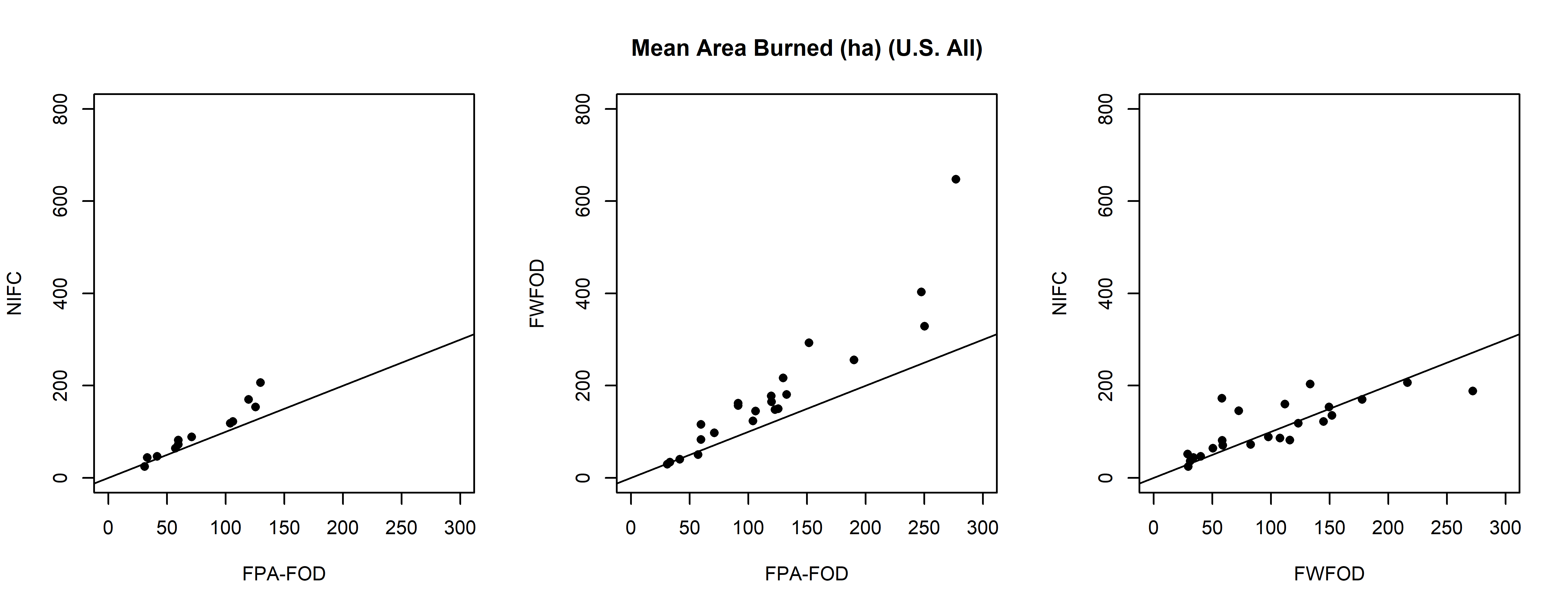
par(oldpar)4.3 Fire size class by year
sizecuts <- c(0.0,0.01,0.1,1,10,100,1000,10000) # c(0.0,0.00001,10,1000000) #
fpafod_lt$sizeclass <- cut(fpafod_lt$AREA_HA,sizecuts)
table(fpafod_lt$sizeclass)
##
## (0,0.01] (0.01,0.1] (0.1,1] (1,10] (10,100] (100,1e+03] (1e+03,1e+04]
## 4018 132305 63052 34490 16423 6772 2621fpafod.tablesize <- table(fpafod_lt$FIRE_YEAR, fpafod_lt$sizeclass)
mosaicplot(fpafod.tablesize, color=TRUE, cex.axis=0.6, las=2, main="fpafod by size, Lightning/Natural Fires")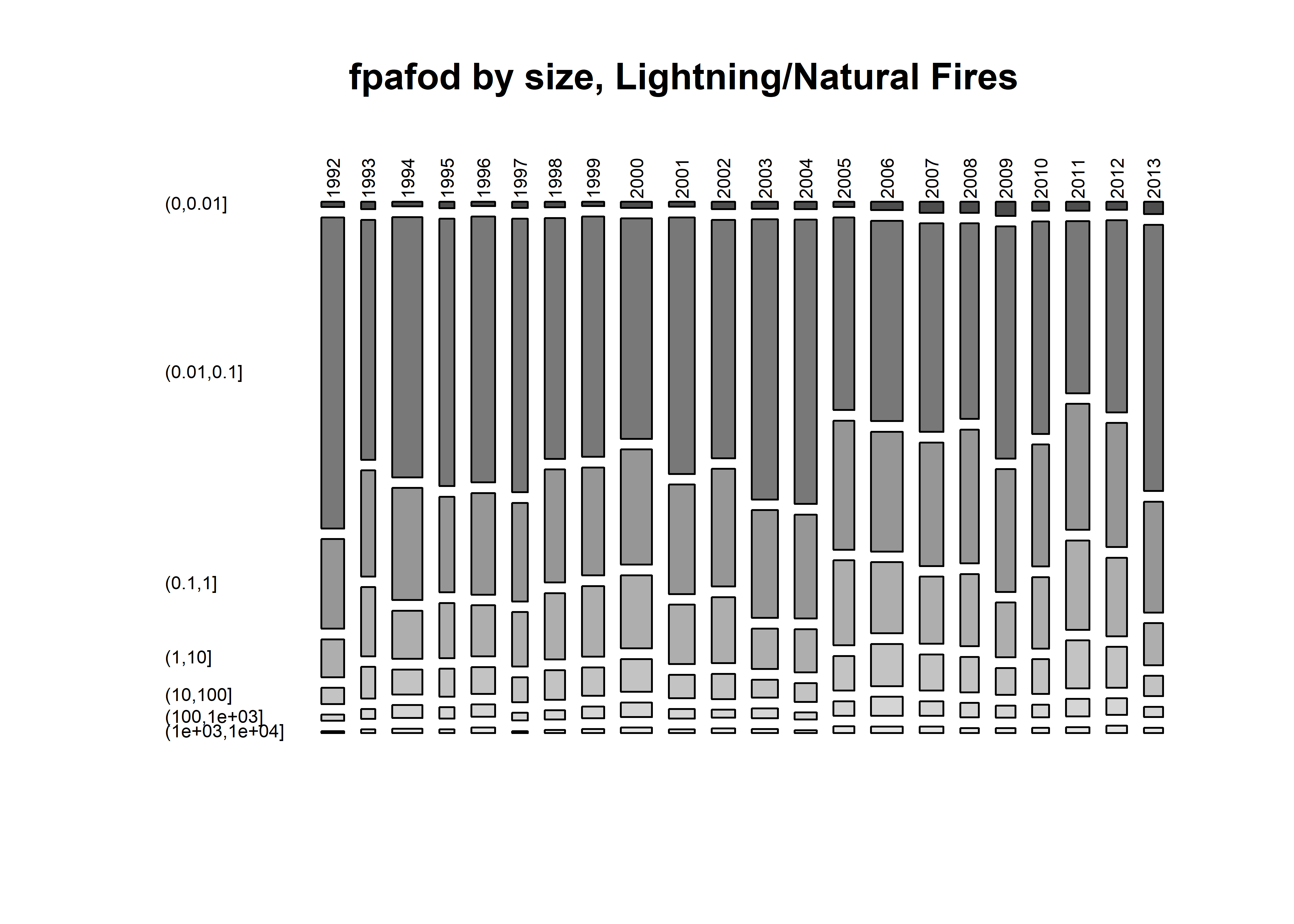
nifc_lt$sizeclass <- cut(nifc_lt$AREA,sizecuts)
table(nifc_lt$sizeclass)
##
## (0,0.01] (0.01,0.1] (0.1,1] (1,10] (10,100] (100,1e+03] (1e+03,1e+04]
## 0 108624 37942 15821 8132 4442 1941nifc.tablesize <- table(nifc_lt$YEAR, nifc_lt$sizeclass)
mosaicplot(nifc.tablesize, color=TRUE, cex.axis=0.6, las=2, main="nifc by size, Lightning/Natural Fires")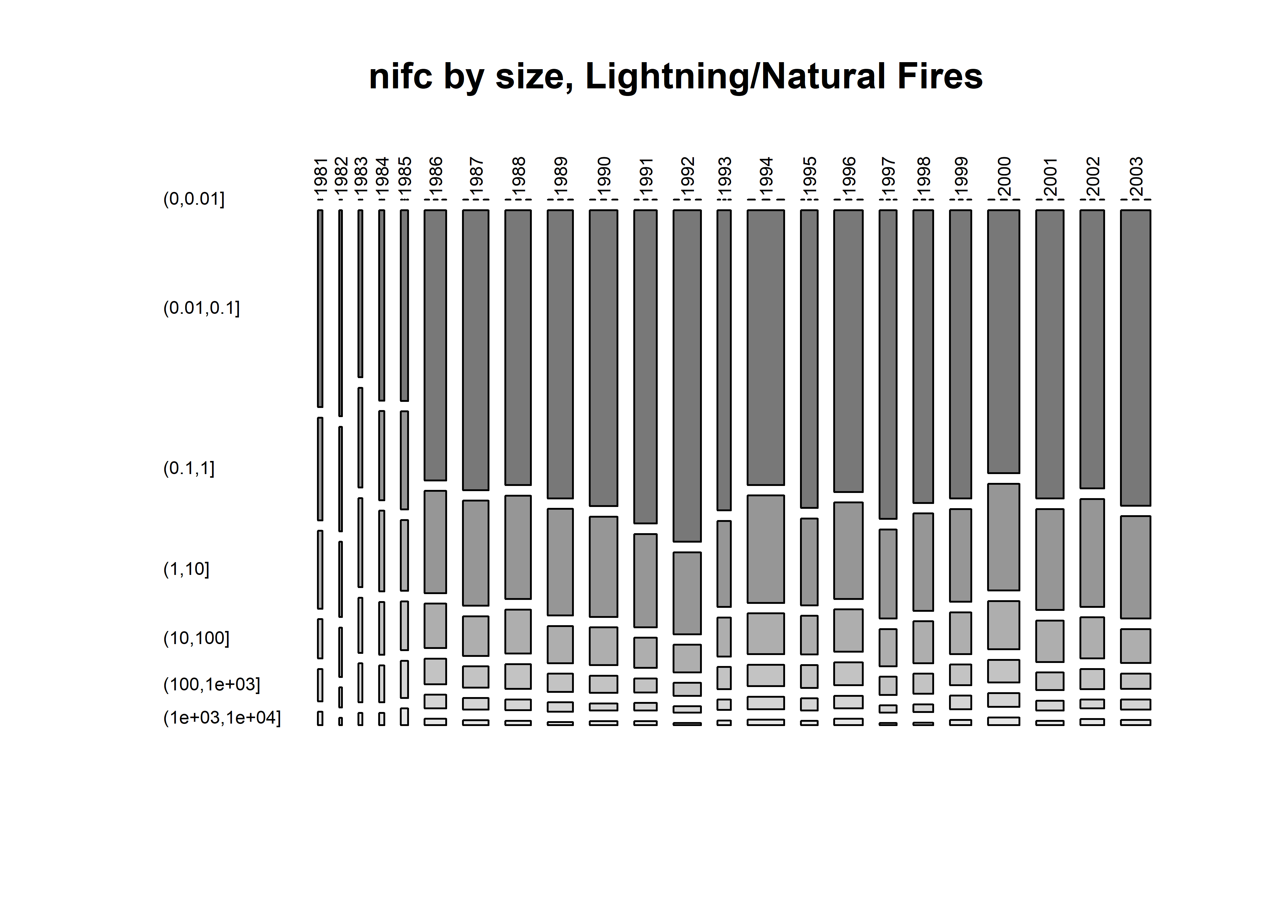
fwfod_lt$sizeclass <- cut(fwfod_lt$AREA,sizecuts)
table(fwfod_lt$sizeclass)
##
## (0,0.01] (0.01,0.1] (0.1,1] (1,10] (10,100] (100,1e+03] (1e+03,1e+04]
## 815 150253 55236 22659 11728 6471 2959fwfod.tablesize <- table(fwfod_lt$startyear, fwfod_lt$sizeclass)
mosaicplot(fwfod.tablesize, color=TRUE, cex.axis=0.6, las=2, main="fwfod by size, Lightning/Natural Fires")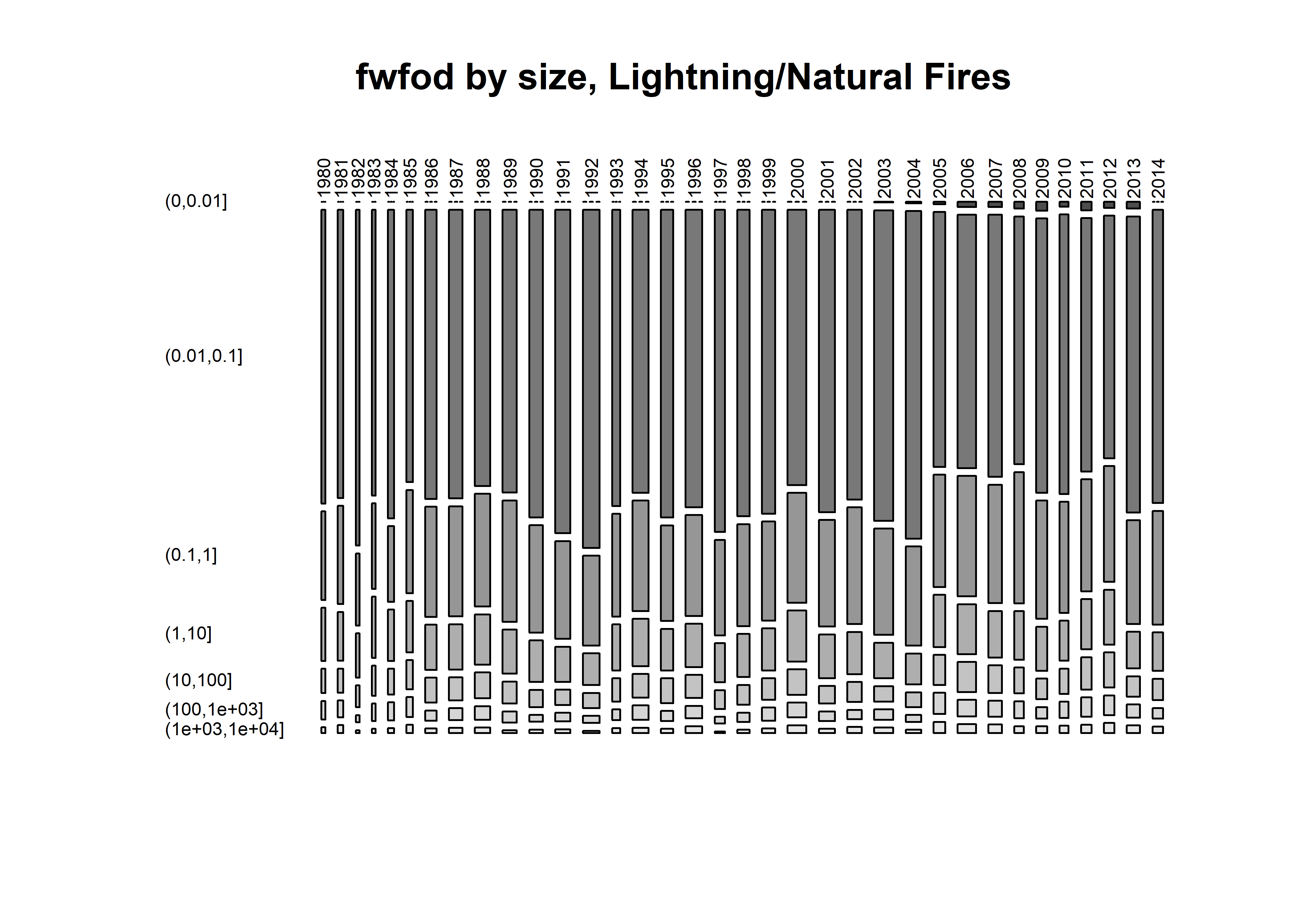
4.4 Fire areas by database
lt_fpafod <- cbind(fpafod_lt$FIRE_YEAR, fpafod_lt$AREA_HA, "FPA-FOD")
lt_nifc <- cbind(nifc_lt$YEAR, nifc_lt$AREA, "NIFC")
lt_fwfod <- cbind(fwfod_lt$startyear, fwfod_lt$AREA, "FWFOD")
lt_fires <-as.data.frame(rbind(lt_fpafod,lt_nifc,lt_fwfod))
names(lt_fires) <- c("Year","AreaHA", "db")
lt_fires[,1] <- as.integer(as.character(lt_fires[,1]))
lt_fires[,2] <- as.numeric(as.character(lt_fires[,2]))
lt_fires <- na.omit(lt_fires)

sizecuts <- c(0.0,0.00001,10,1000000) #
lt_fires$sizeclass <- cut(lt_fires$AreaHA,sizecuts)
table(lt_fires$sizeclass)
##
## (0,1e-05] (1e-05,10] (10,1e+06]
## 0 625211 63305lt_tablesize <- table(lt_fires$db, lt_fires$sizeclass)
mosaicplot(lt_tablesize, color=TRUE, cex.axis=0.6, las=2,
main="Lightning/Natural Fires -- Size (ha) by Database")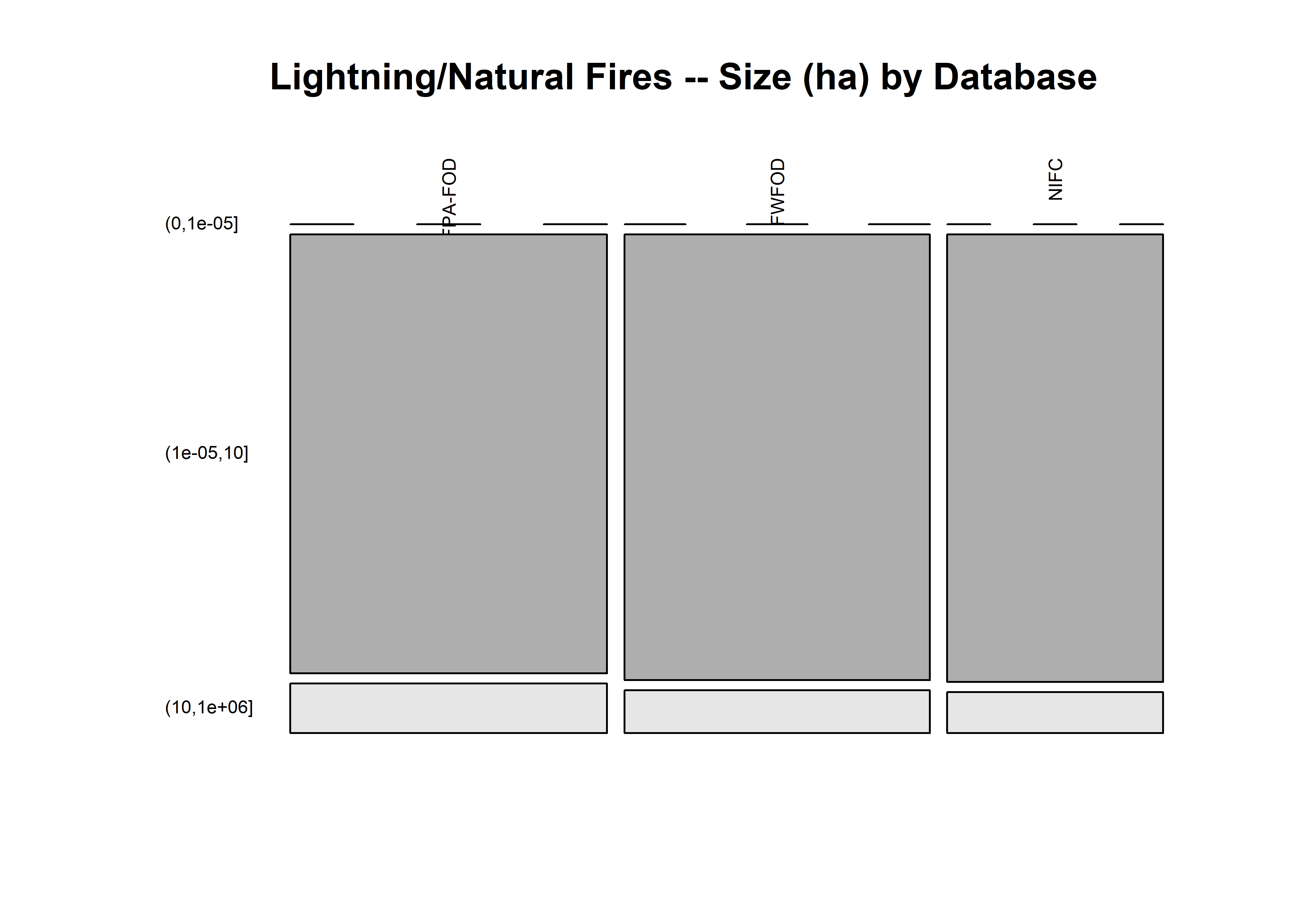
sizecuts <- c(0.0,0.01,0.1,1,10,100,1000,10000) # c(0.0,0.00001,10,1000000) #
lt_fires$sizeclass <- cut(lt_fires$AreaHA,sizecuts)
table(lt_fires$sizeclass)
##
## (0,0.01] (0.01,0.1] (0.1,1] (1,10] (10,100] (100,1e+03] (1e+03,1e+04]
## 4833 391180 156229 72969 36283 17685 7521lt_tablesize <- table(lt_fires$db, lt_fires$sizeclass)
mosaicplot(lt_tablesize, color=TRUE, cex.axis=0.6, las=2,
main="Lightning/Natural Fires -- Size (ha) by Database")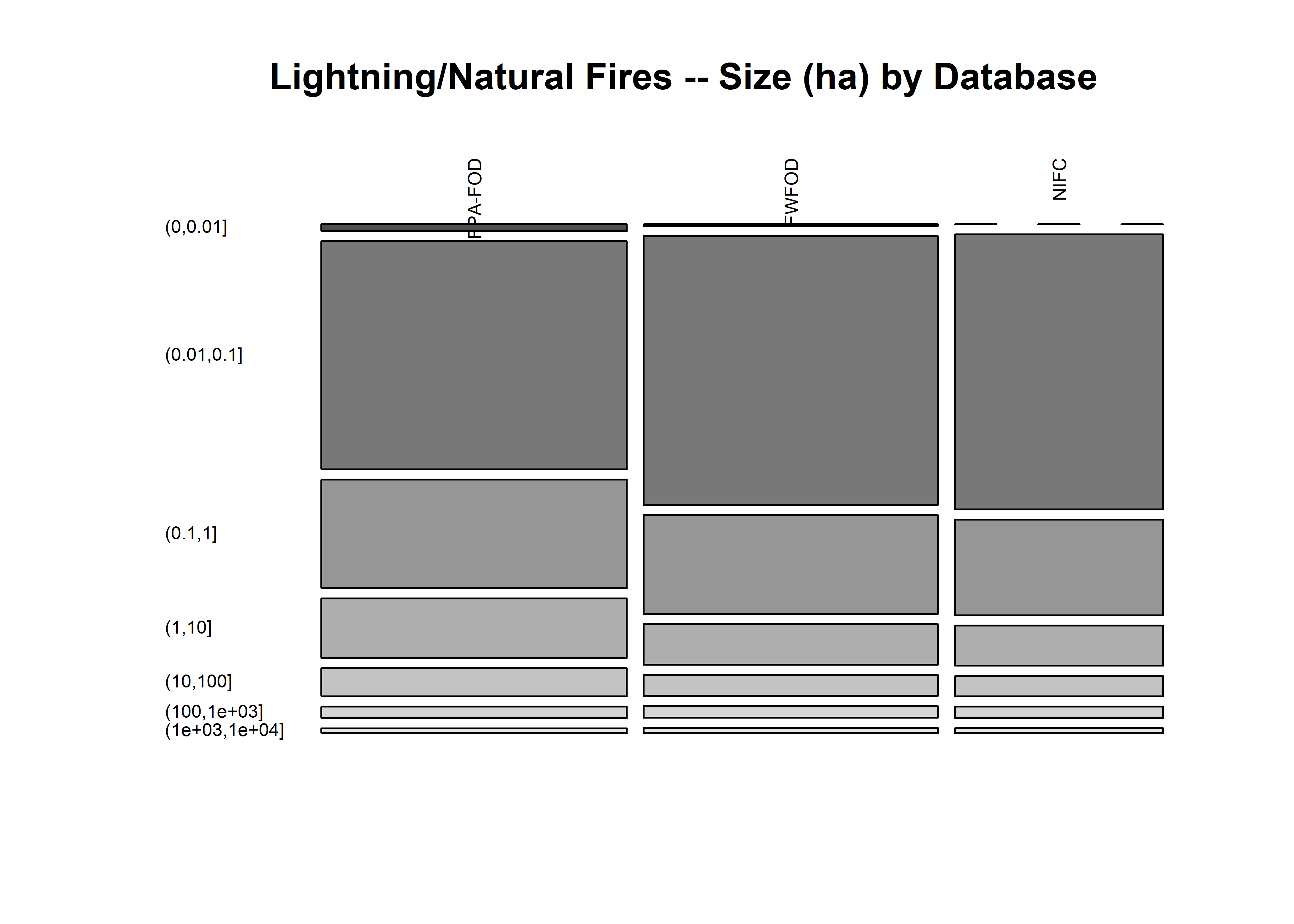
4.5 Fire frequency by month and year
fpafod.tablemon <- table(fpafod_lt$FIRE_YEAR,
  fpafod_lt$startmon)
mosaicplot(fpafod.tablemon, color=monthcolors, cex.axis=0.6, las=3, main="FPA-FOD, Lightning/Natural Fires, All Agencies")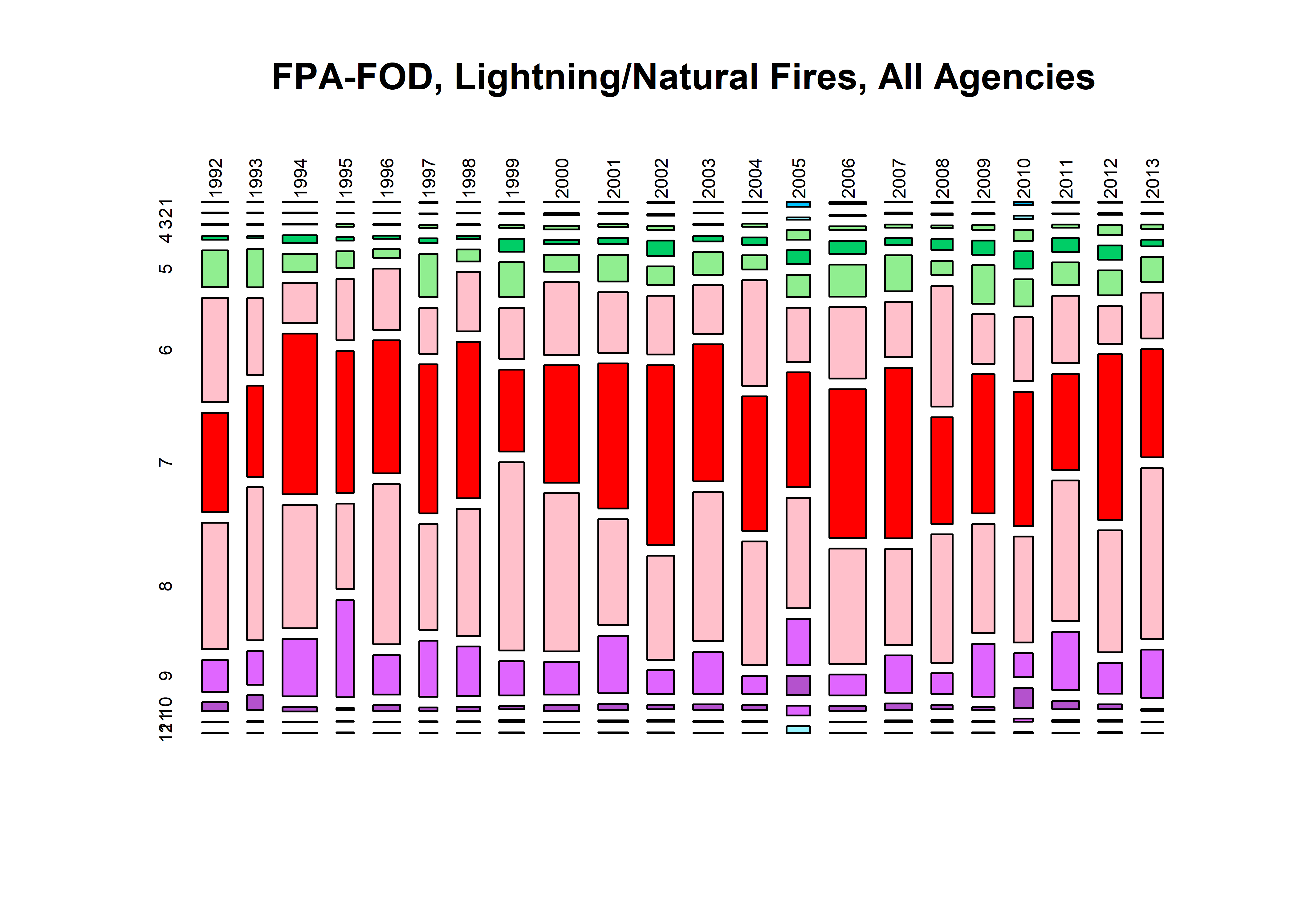
nifc.tablemon <- table(nifc_lt$YEAR, nifc_lt$startmon)
mosaicplot(nifc.tablemon, color=monthcolors, cex.axis=0.6, las=3, main="NIFC, Lightning/Natural Fires, All Agencies")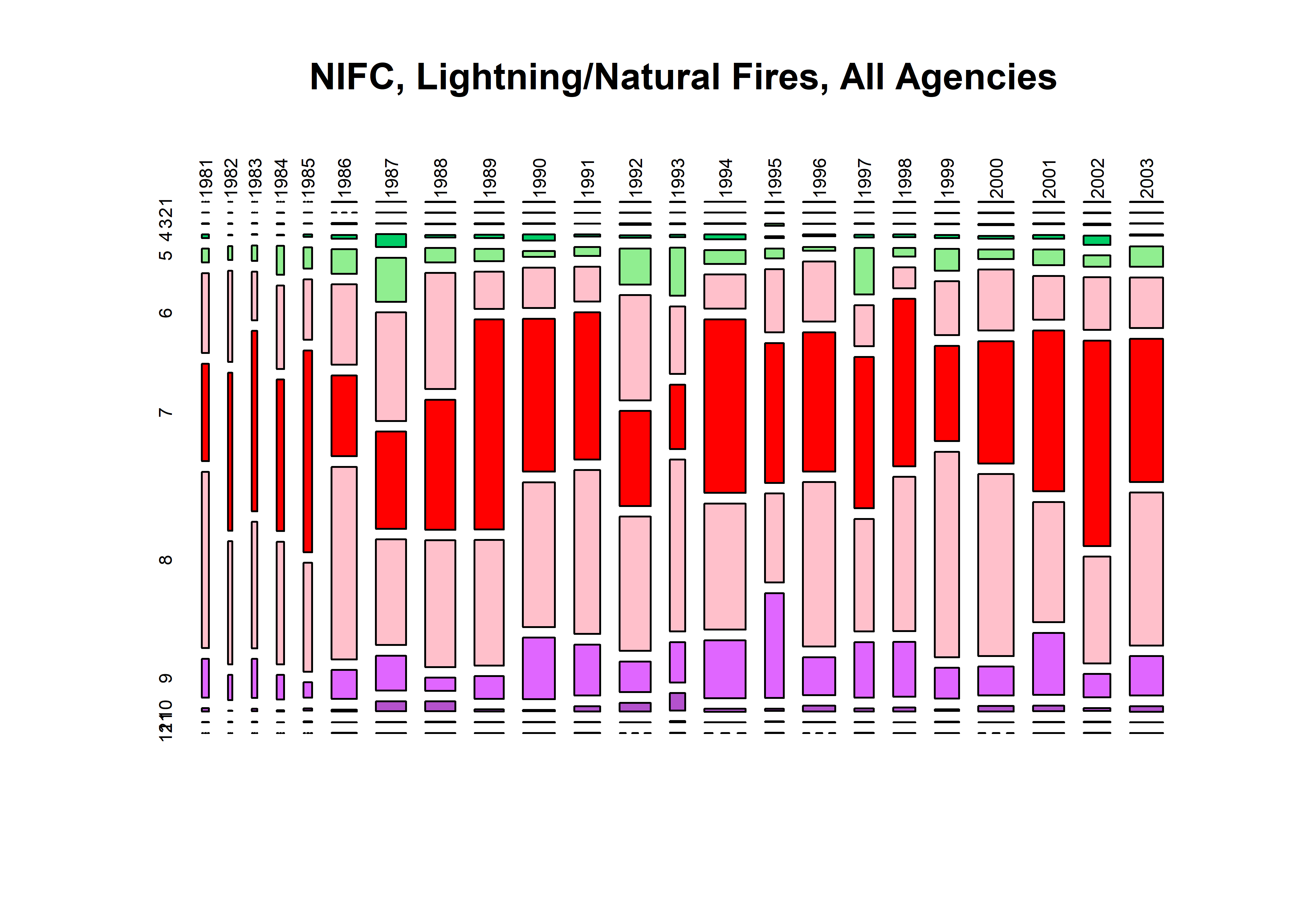
fwfod.tablemon <- table(fwfod_lt$startyear, fwfod_lt$startmon)
mosaicplot(fwfod.tablemon, color=monthcolors, cex.axis=0.6, las=3, main="FWFOD, Lightning/Natural Fires, All Agencies")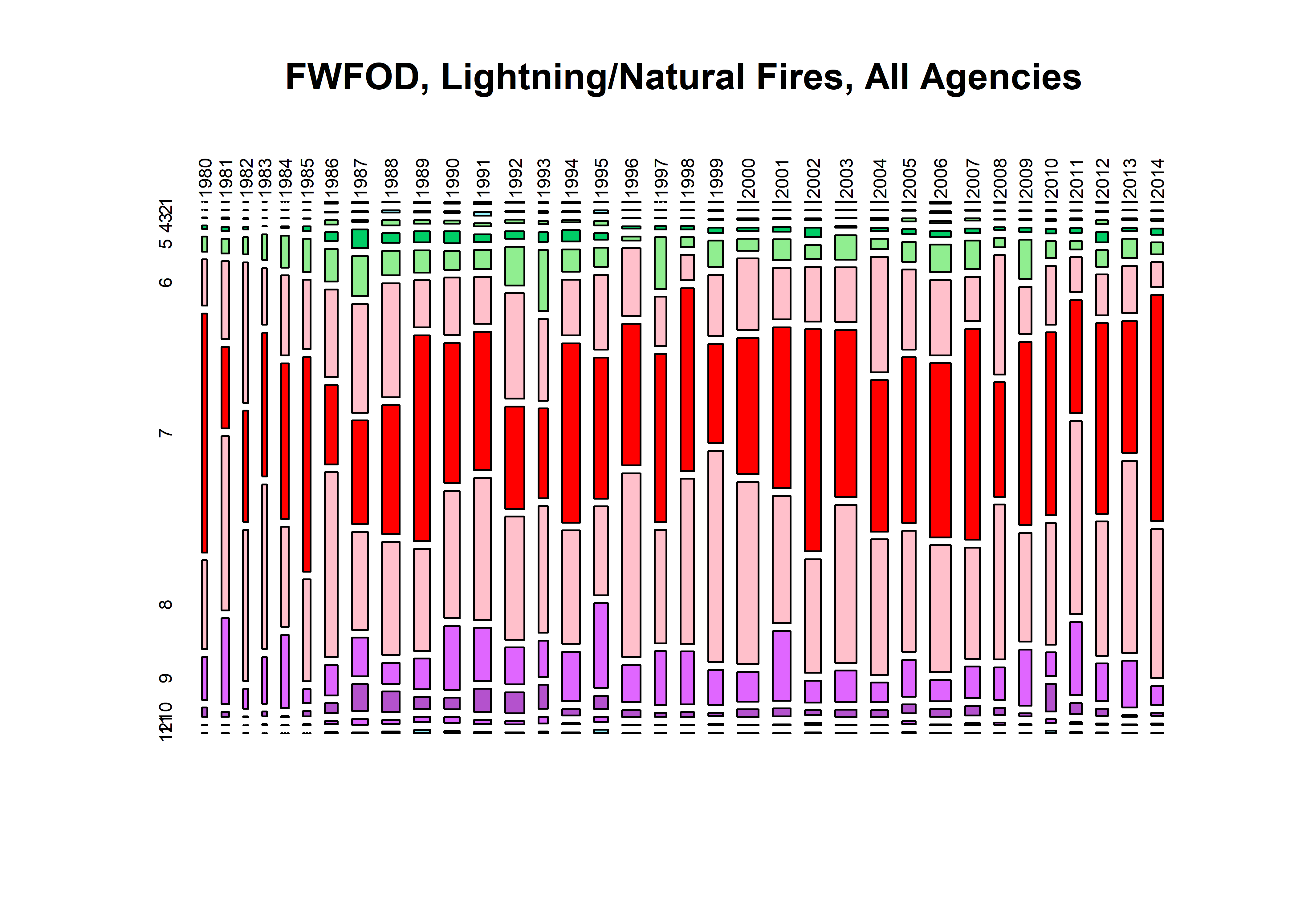
4.6 U.S. Forest Service
table(fpafod_lt$FIRE_YEAR[fpafod_lt$NWCG_REPORTING_AGENCY =="FS"])##
## 1992 1993 1994 1995 1996 1997 1998 1999 2000 2001 2002 2003 2004 2005 2006 2007 2008 2009 2010 2011 2012
## 6816 2963 9338 3898 6567 4000 4947 4912 6827 5935 5195 6850 5001 3584 6473 4716 3694 3939 2842 3642 3417
## 2013
## 4334table(nifc_lt$YEAR[nifc_lt$AGENCY_COD=="USFS"])##
## 1981 1983 1984 1985 1986 1987 1988 1989 1990 1991 1992 1993 1994 1995 1996 1997 1998 1999 2000 2001 2002
## 4 56 111 47 5662 6993 6575 6907 7333 5778 6915 3015 9494 3942 6613 4021 4981 4941 6892 5990 5180
## 2003
## 6820table(fwfod_lt$startyear[fwfod_lt$ORGANIZATI=="FS"])##
## 1980 1981 1982 1983 1984 1985 1986 1987 1988 1989 1990 1991 1992 1993 1994 1995 1996 1997 1998 1999 2000
## 1695 1850 1453 1296 2219 2030 5070 6135 6296 6352 6000 6674 7373 3321 6062 5493 6615 4021 4987 4972 6872
## 2001 2002 2003 2004 2005 2006 2007 2008 2009 2010 2011 2012 2013 2014
## 6007 5254 6887 5015 3619 6514 4705 3739 3883 2815 3696 3374 4153 3696fpafod.tablemon <- table(fpafod_lt$FIRE_YEAR[fpafod_lt$NWCG_REPORTING_AGENCY == "FS" &
fpafod_lt$STAT_CAUSE_CODE == 1], fpafod_lt$startmon[fpafod_lt$NWCG_REPORTING_AGENCY == "FS" &
fpafod_lt$STAT_CAUSE_CODE == 1])
mosaicplot(fpafod.tablemon, color=monthcolors, cex.axis=0.6, las=3, main="FPA-FOD, Lightning/Natural Fires, FS")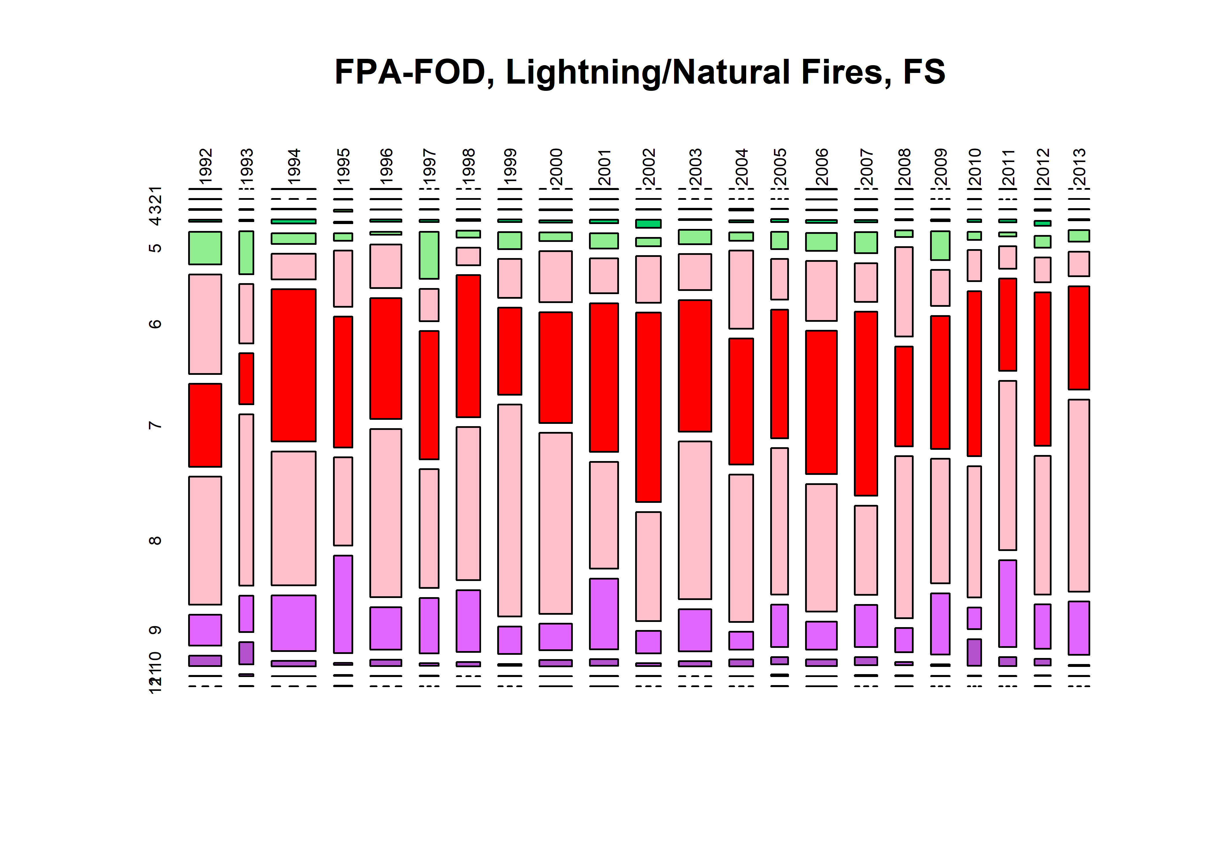
nifc.tablemon <- table(nifc_lt$YEAR[nifc_lt$AGENCY_COD== "USFS"],
  nifc_lt$startmon[nifc_lt$AGENCY_COD== "USFS"])
mosaicplot(nifc.tablemon, color=monthcolors, cex.axis=0.6, las=3, main="NIFC, Lightning/Natural Fires, FS")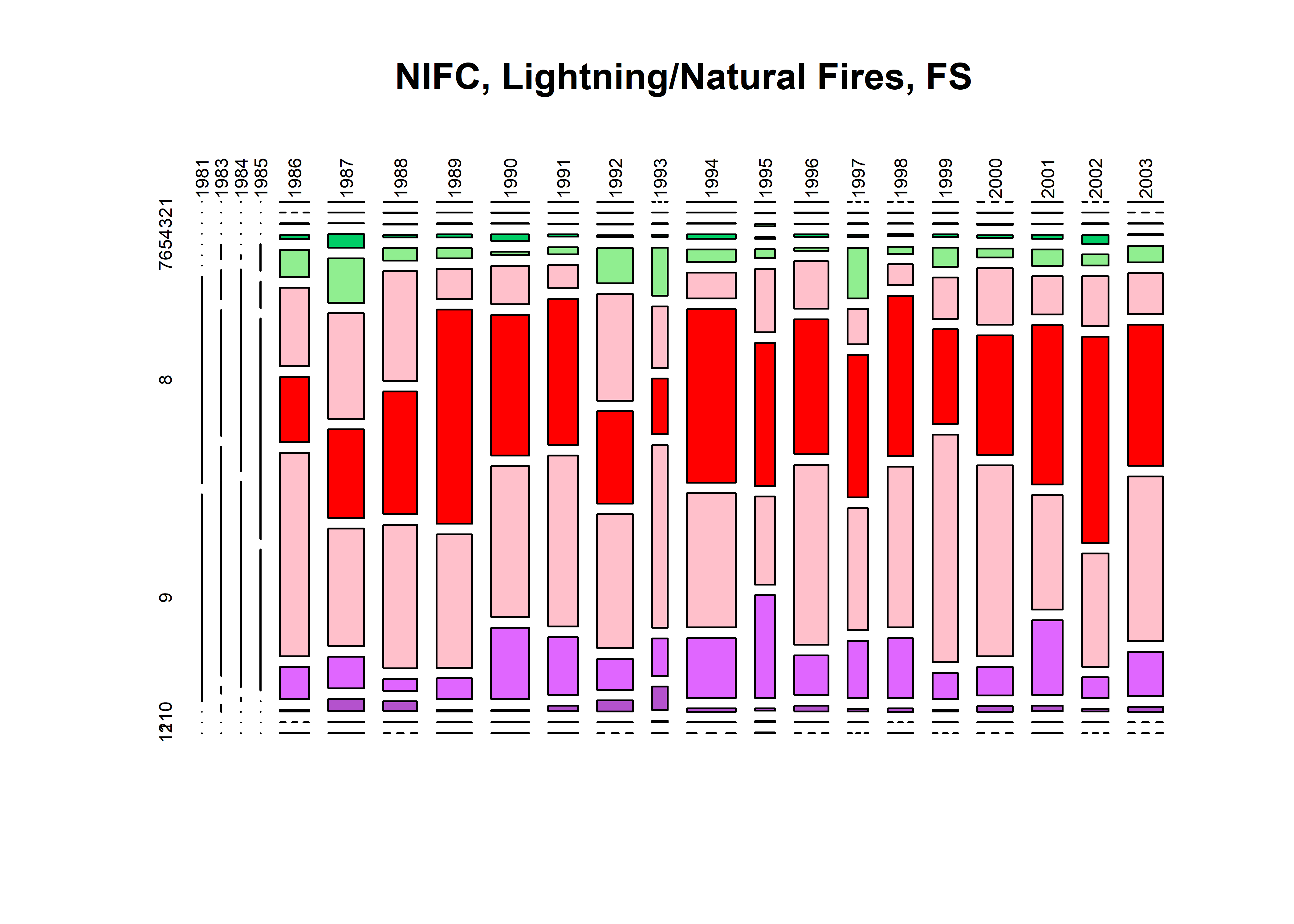
fwfod.tablemon <- table(fwfod_lt$startyear[fwfod_lt$ORGANIZATI== "FS"],
  fwfod_lt$startmon[fwfod_lt$ORGANIZATI== "FS"])
mosaicplot(fwfod.tablemon, color=monthcolors, cex.axis=0.6, las=3, main="FWFOD, Lightning/Natural Fires, FS")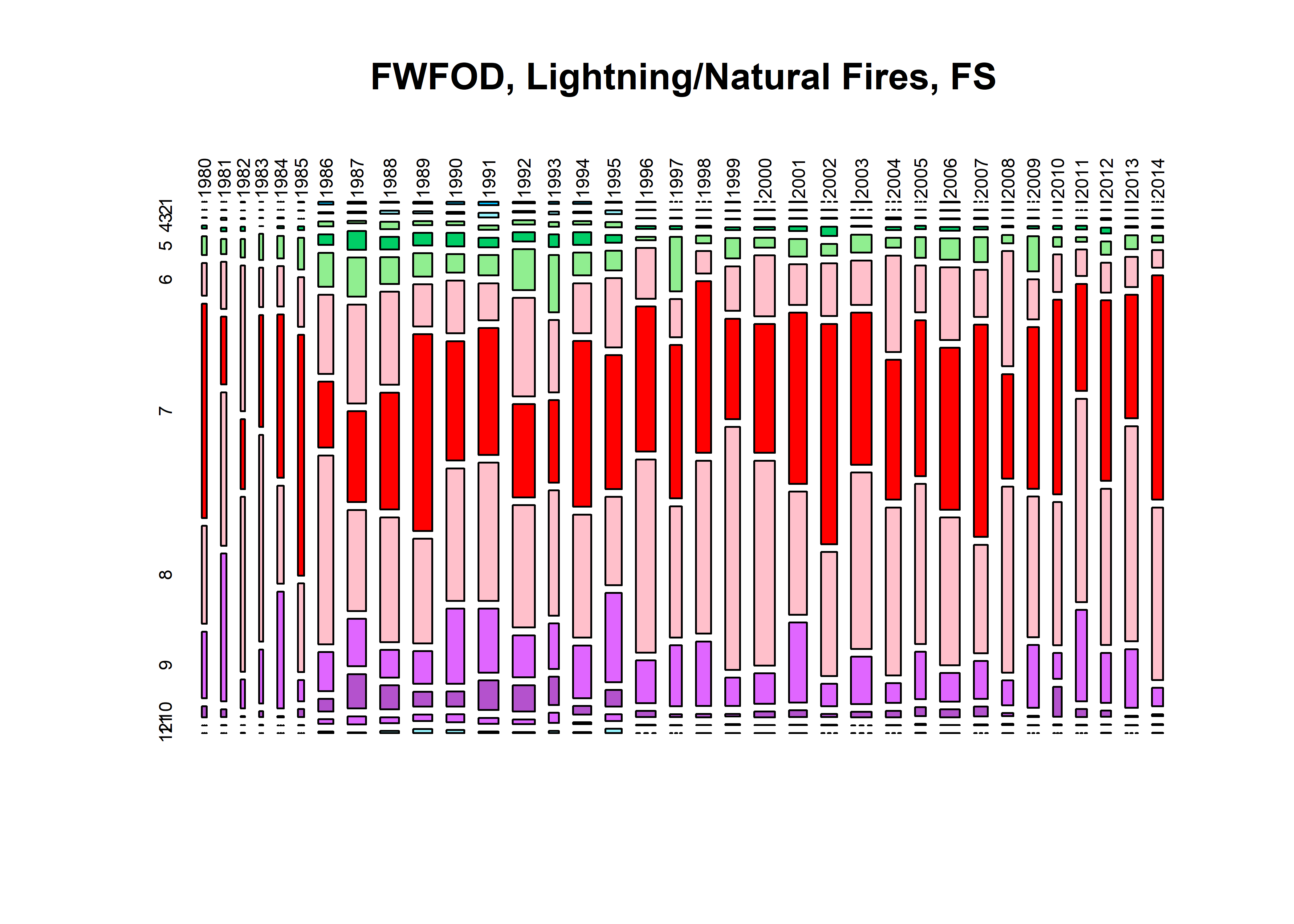
hist(nifc_lt$YEAR, xlim=c(1980,2015), ylim=c(0,30000),
   breaks=seq(1979.5,2014.5,by=1), col="lightblue", border="blue", main="Lightning/Natural Fires")
hist(fpafod_lt$FIRE_YEAR, xlim=c(1980,2015), ylim=c(0,15000),
  breaks=seq(1979.5,2014.5,by=1), xlab="Year", col="pink", border="red", add=TRUE)
hist(fwfod_lt$startyear, xlim=c(1980,2015), ylim=c(0,15000),
  breaks=seq(1979.5,2014.5,by=1), add=TRUE,  border="purple")
hist(nifc_lt$YEAR, xlim=c(1980,2015), ylim=c(0,15000),
   breaks=seq(1979.5,2014.5,by=1), border="blue", add=TRUE)
legend("topleft", legend=c("FPA-FOD","NIFC","FWFOD"), lwd=2, col=c("red","blue","purple"))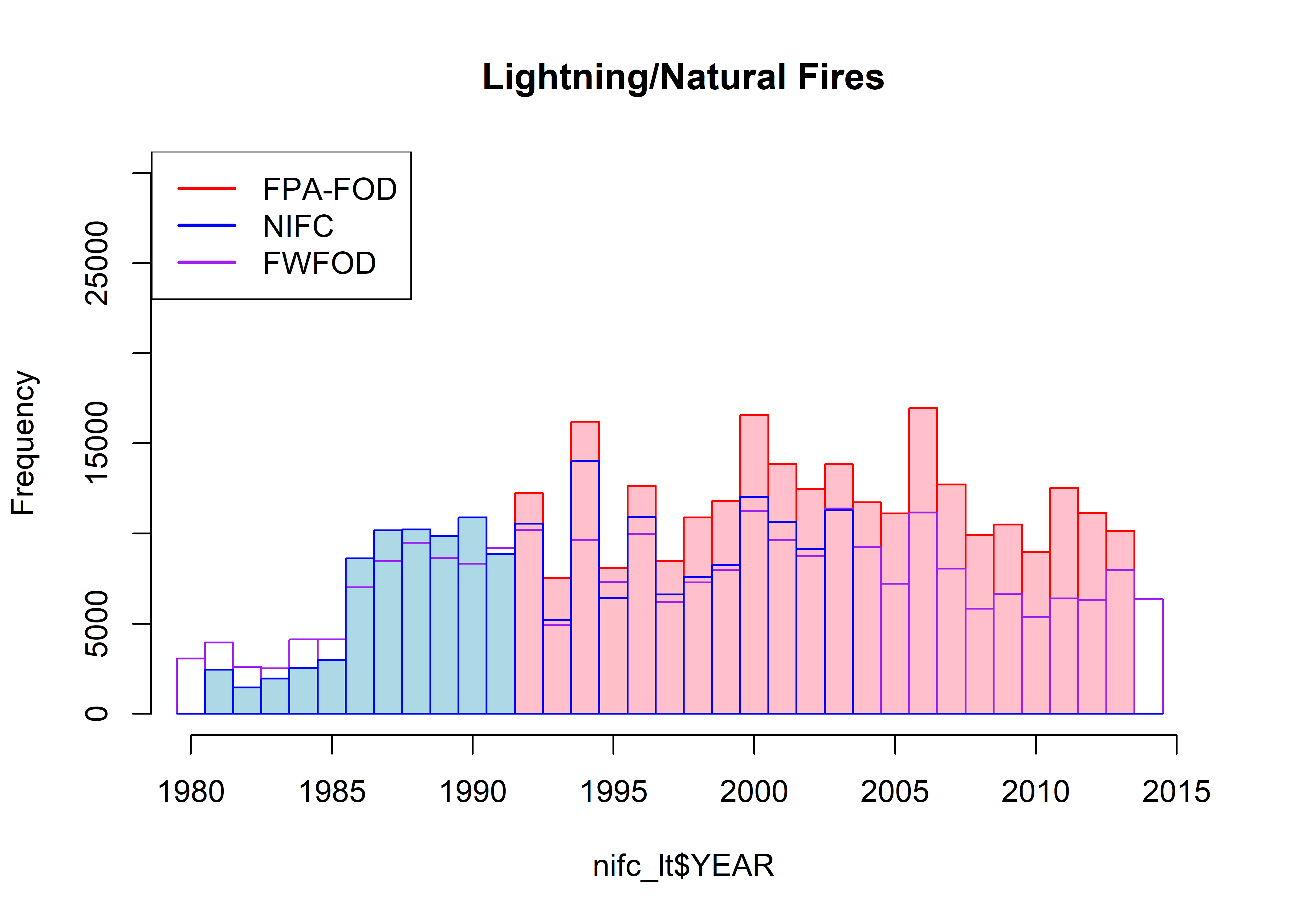
hist(nifc_lt$YEAR[nifc_lt$AGENCY_COD=="USFS"], xlim=c(1980,2015), ylim=c(0,15000),
   breaks=seq(1979.5,2014.5,by=1), col="lightblue", border="blue", main="Lightning/Natural Fires, USFS")
hist(fpafod_lt$FIRE_YEAR[fpafod_lt$NWCG_REPORTING_AGENCY =="FS"],
  xlim=c(1980,2015), ylim=c(0,120000), breaks=seq(1979.5,2014.5,by=1), xlab="Year", col="pink", border="red",
  add=TRUE)
hist(fwfod_lt$startyear[fwfod_lt$ORGANIZATI=="FS"], xlim=c(1980,2015), ylim=c(0,15000),
  breaks=seq(1979.5,2014.5,by=1), add=TRUE, border="purple")
hist(nifc_lt$YEAR[nifc_lt$AGENCY_COD=="USFS"], xlim=c(1980,2015), ylim=c(0,15000),
   breaks=seq(1979.5,2014.5,by=1), border="blue", add=TRUE)
legend("topleft", legend=c("FPA-FOD","NIFC","FWFOD"), lwd=2, col=c("red","blue","purple"))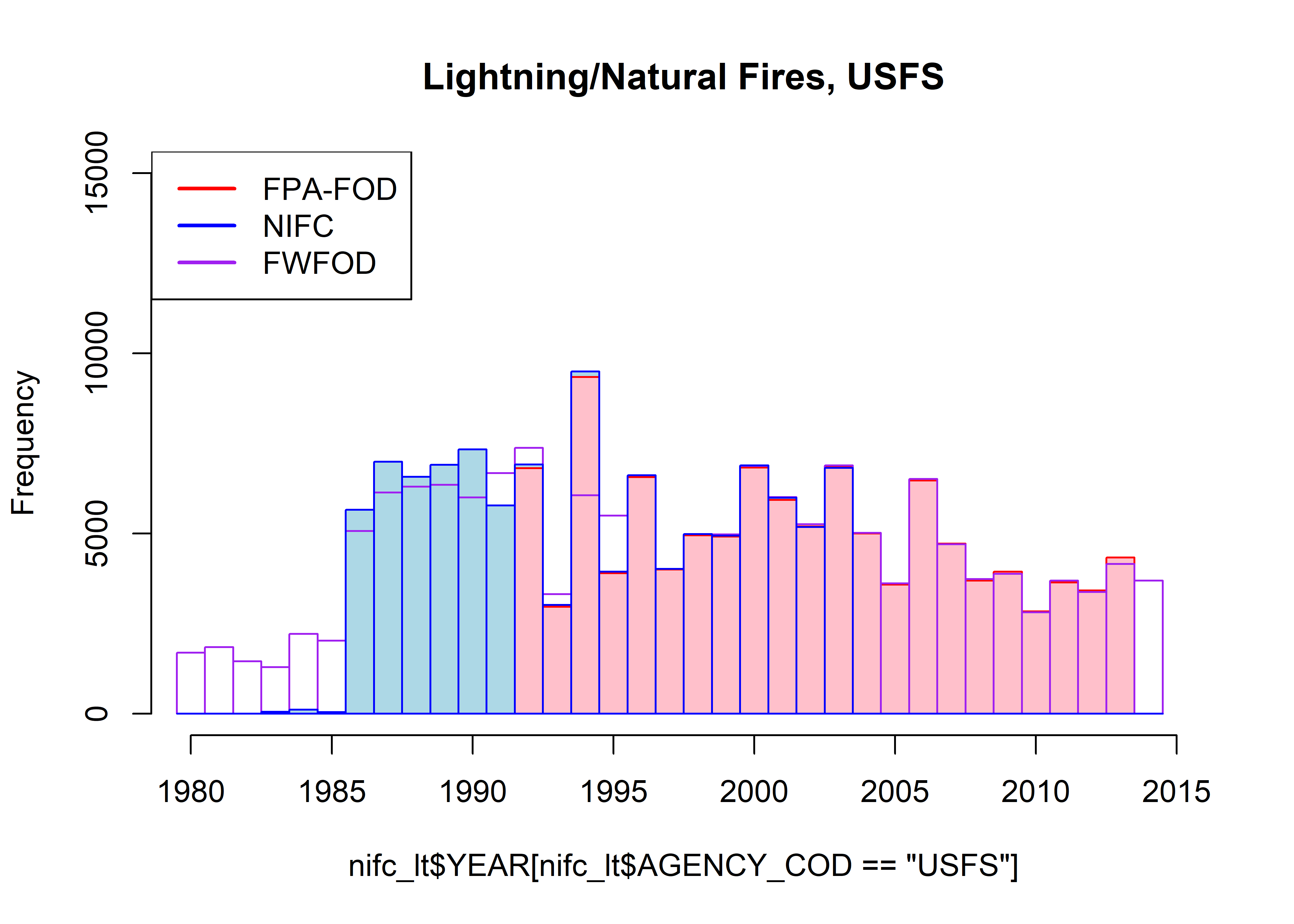
5 Compare FPA-FOD, FWFOD, and NIFC – Human-started fires
Get Human-started fires
fpafod_hu <- fpafod[fpafod$STAT_CAUSE_CODE >= 2 && fpafod$STAT_CAUSE_CODE < 13, ]
nifc_hu <- nifc[as.numeric(nifc$GENERAL_CA) >= 2, ]
fwfod_hu <- fwfod[fwfod$CAUSE == "Human", ]
5.1 Maps
library(maps)
plot(fpafod_hu$LATITUDE ~ fpafod_hu$LONGITUDE, ylim=c(17,80), xlim=c(-180,-55), type="n",
  xlab="Longitude", ylab="Latitude", main="FPA-FOD -- Human Fires")
map("world", add=TRUE, lwd=2, col="gray")
points(fpafod_hu$LATITUDE ~ fpafod_hu$LONGITUDE, pch=16, cex=0.2, col="red")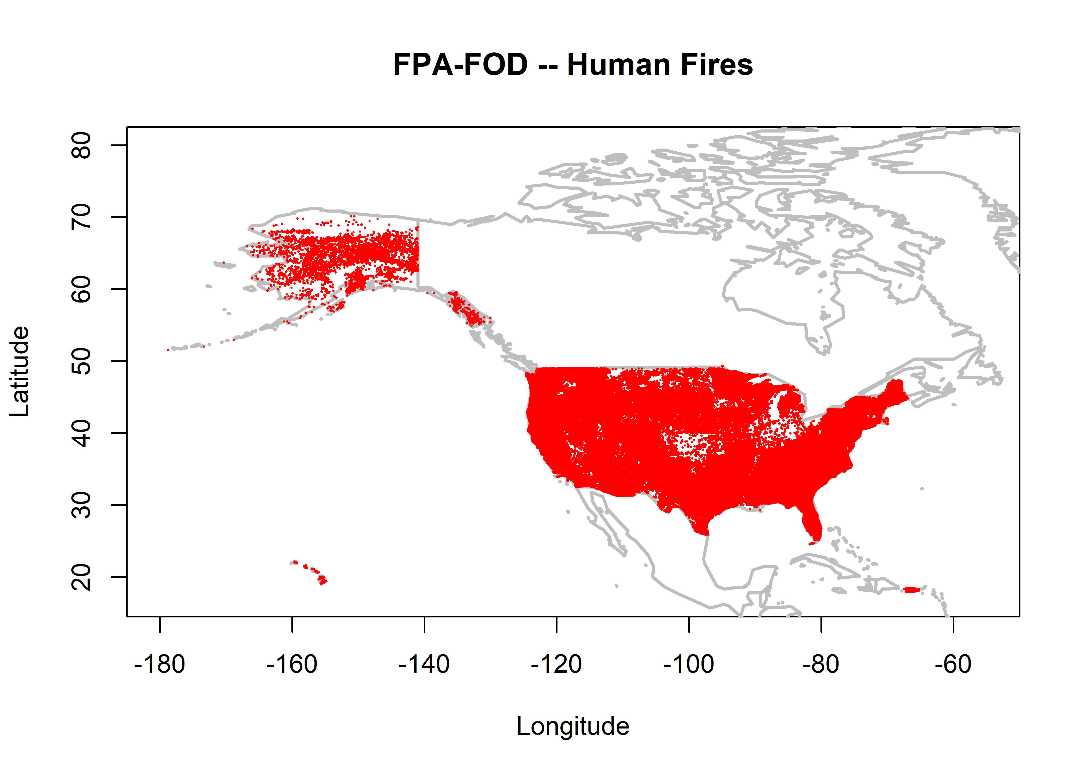
plot(nifc_hu$LATITUDE ~ nifc_hu$LONGITUDE, ylim=c(17,80), xlim=c(-180,-55), type="n",
  xlab="Longitude", ylab="Latitude", main="NIFC -- Human Fires")
map("world", add=TRUE, lwd=2, col="gray")
points(nifc_hu$LATITUDE ~ nifc_hu$LONGITUDE, pch=16, cex=0.2, col="red")
plot(fwfod_hu$DLATITUDE ~ fwfod_hu$DLONGITUDE, ylim=c(17,80), xlim=c(-180,-55), type="n",
  xlab="Longitude", ylab="Latitude", main="FWFOD -- Human Fires")
map("world", add=TRUE, lwd=2, col="gray")
points(fwfod_hu$DLATITUDE ~ fwfod_hu$DLONGITUDE, pch=16, cex=0.2, col="red")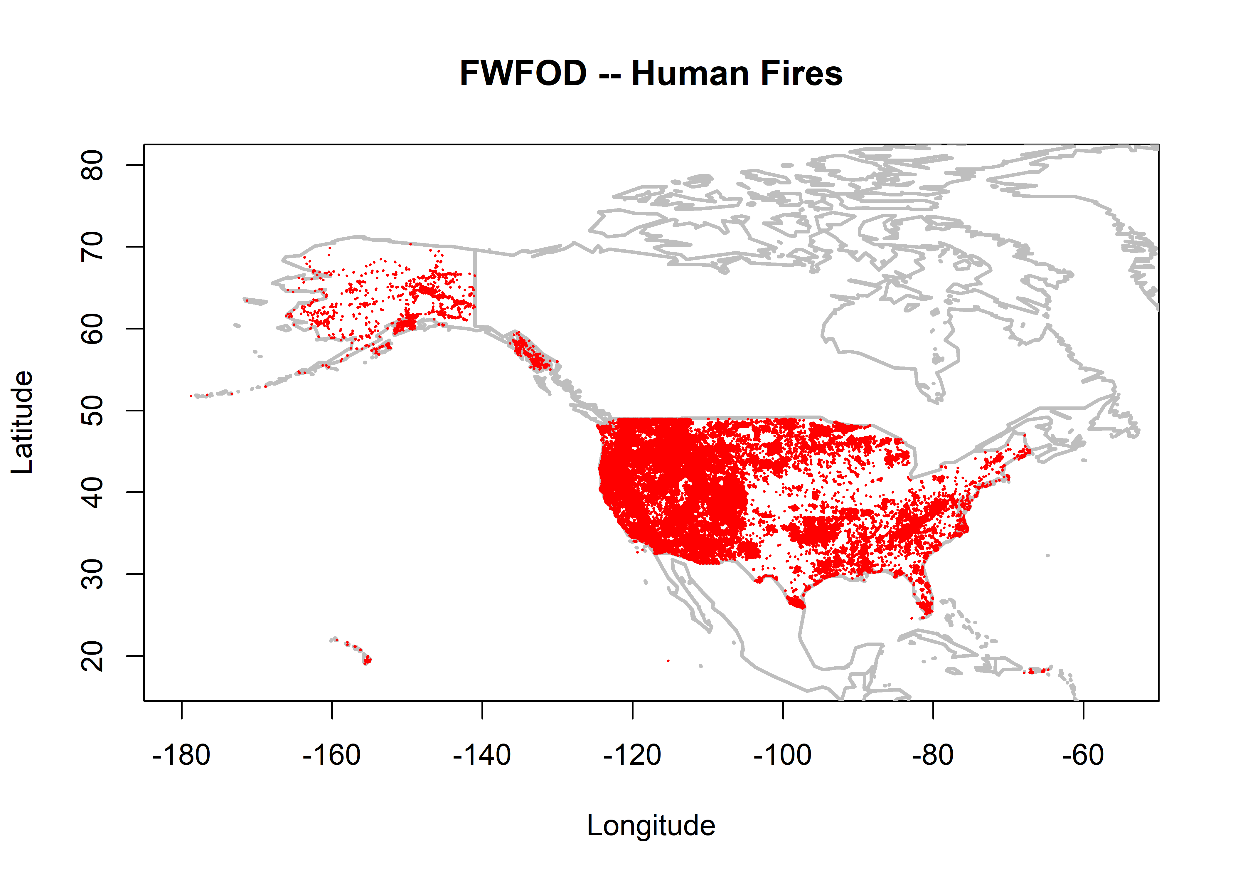
5.2 Time series – number and area
5.2.1 Total number of fires
Plot the fire count data.
fpafod_hu_num <- hist(fpafod_hu$FIRE_YEAR, breaks=seq(1979.5,2015.5, by=1), plot = FALSE)
nifc_hu_num <- hist(nifc_hu$YEAR, breaks=seq(1979.5,2015.5, by=1), plot = FALSE)
fwfod_hu_num <- hist(fwfod_hu$startyear, breaks=seq(1979.5,2015.5,by=1), plot = FALSE)

all_num_hu <- data.frame(fpafod_hu_num$mids, fpafod_hu_num$counts, nifc_hu_num$counts, fwfod_hu_num$counts)
all_num_hu[all_num_hu == 0] <- NA
names(all_num_hu) <- c("Year", "fpafod_hu_num", "nifc_hu_num", "fwfod_hu_num")
all_num_hu
## Year fpafod_hu_num nifc_hu_num fwfod_hu_num
## 1 1980 NA NA 5641
## 2 1981 NA 4735 6118
## 3 1982 NA 3030 3467
## 4 1983 NA 4167 3720
## 5 1984 NA 5420 4806
## 6 1985 NA 7280 6062
## 7 1986 NA 16920 8272
## 8 1987 NA 20980 10743
## 9 1988 NA 21076 10231
## 10 1989 NA 19152 9034
## 11 1990 NA 19615 9333
## 12 1991 NA 18498 7933
## 13 1992 67964 21228 9006
## 14 1993 62022 15985 9280
## 15 1994 75989 25869 13962
## 16 1995 71496 18370 9299
## 17 1996 75604 21931 10101
## 18 1997 61472 15031 7886
## 19 1998 68388 17826 10489
## 20 1999 89398 20731 13574
## 21 2000 96454 23126 11733
## 22 2001 86069 21588 11593
## 23 2002 75136 20490 11810
## 24 2003 67380 19716 10690
## 25 2004 68616 NA 9886
## 26 2005 87391 NA 12130
## 27 2006 113242 NA 13269
## 28 2007 94681 NA 12195
## 29 2008 84654 NA 9705
## 30 2009 77262 NA 9041
## 31 2010 78485 NA 9499
## 32 2011 89897 NA 9307
## 33 2012 71768 NA 9935
## 34 2013 64108 NA 8294
## 35 2014 NA NA 8931
## 36 2015 NA NA NATime series plots of the numbers of fires:
plot(all_num_hu$fpafod_hu_num ~ all_num_hu$Year, type="o", col="red", pch=16, xlim=c(1980,2015),
     ylim=c(0,120000),xlab="Year", ylab="Total Number of Fires",
     main="Total Number of Fires (U.S. Human)", lwd=2)
lines(all_num_hu$nifc_hu_num ~ all_num_hu$Year, type="o", col="blue", pch=16, lwd=2)
lines(all_num_hu$fwfod_hu_num ~ all_num_hu$Year, type="o", col="purple", pch=16, lwd=2)
legend("topleft", legend=c("FPA-FOD","NIFC","FWFOD"), lwd=2, col=c("red","blue","purple"))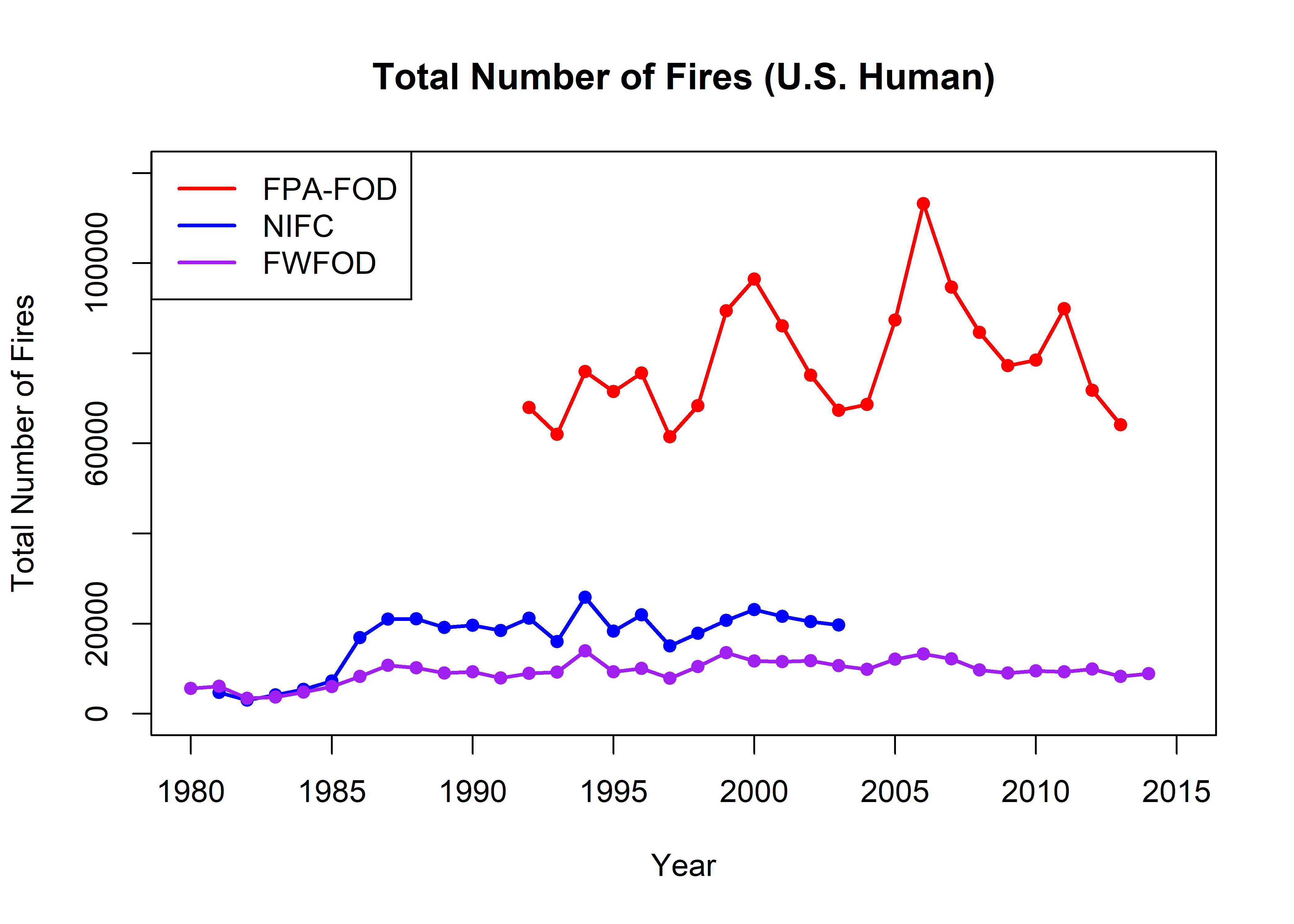
Scatter plots that compare the three different data sets:
oldpar <- par(mfrow=c(1,3))
plot(all_num_hu$fpafod_hu_num, all_num_hu$nifc_hu_num, xlim=c(0,120000), ylim=c(0,120000), pch=16,
     xlab="FPA-FOD", ylab="NIFC"); abline(0,1)
plot(all_num_hu$fpafod_hu_num, all_num_hu$fwfod_hu_num, xlim=c(0,120000), ylim=c(0,120000), pch=16,
     xlab="FPA-FOD", ylab="FWFOD", main="Total Number of Fires (U.S. Human)"); abline(0,1)
plot(all_num_hu$fwfod_hu_num, all_num_hu$nifc_hu_num, xlim=c(0,120000), ylim=c(0,120000), pch=16,
     xlab="FWFOD", ylab="NIFC"); abline(0,1)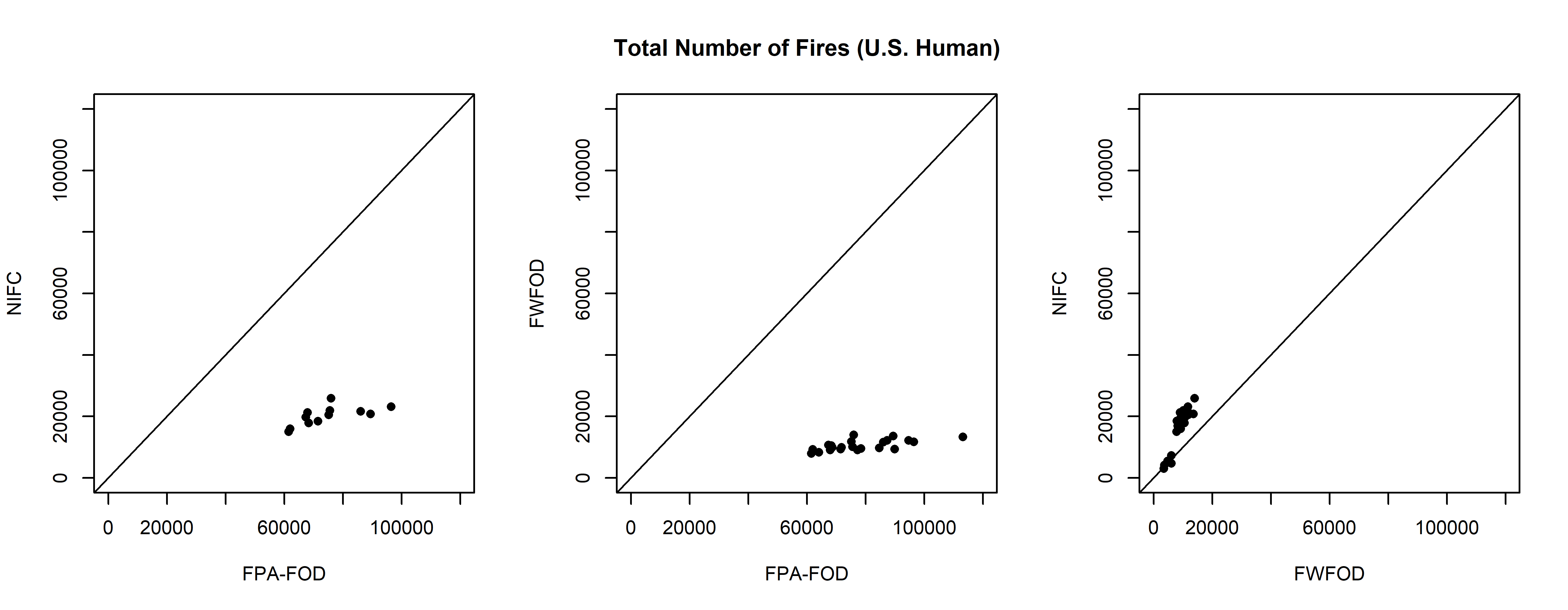
par(oldpar)5.2.2 Total area burned
Get time series of total area burned.
all_totalarea_hu <- data.frame(matrix(nrow = 36, ncol = 4))
names(all_totalarea_hu) <- c("Year", "fpafod_hu_totalarea", "nifc_hu_totalarea",
      "fwfod_hu_totalarea")
all_totalarea_hu["Year"] <- seq(1980, 2015, by=1)

fpafod_hu_total_by_year <- tapply(fpafod_hu$AREA_HA, fpafod_hu$FIRE_YEAR, sum)
fpafod_hu_year <- as.numeric(unlist(dimnames(fpafod_hu_total_by_year)))
fpafod_hu_total_by_year <- as.numeric(fpafod_hu_total_by_year)
all_totalarea_hu$fpafod_hu_totalarea[fpafod_hu_year-1980+1] <- fpafod_hu_total_by_year

fwfod_hu_total_by_year <- tapply(fwfod_hu$AREA, fwfod_hu$startyear, sum)
fwfod_hu_year <- as.numeric(unlist(dimnames(fwfod_hu_total_by_year)))
fwfod_hu_total_by_year <- as.numeric(fwfod_hu_total_by_year)
all_totalarea_hu$fwfod_hu_totalarea[fwfod_hu_year-1980+1] <- fwfod_hu_total_by_year

nifc_hu_size_year <- na.omit(cbind(nifc_hu$AREA,nifc_hu$YEAR))
nifc_hu_total_by_year <- tapply(nifc_hu_size_year[,1],nifc_hu_size_year[,2], sum)
nifc_hu_year <- as.numeric(unlist(dimnames(nifc_hu_total_by_year)))
nifc_hu_total_by_year <- as.numeric(nifc_hu_total_by_year)
all_totalarea_hu$nifc_hu_totalarea[nifc_hu_year-1980+1] <- nifc_hu_total_by_year

all_totalarea_hu
## Year fpafod_hu_totalarea nifc_hu_totalarea fwfod_hu_totalarea
## 1 1980 NA NA 249786.48
## 2 1981 NA 761427.6 329478.51
## 3 1982 NA 161320.7 90566.95
## 4 1983 NA 476053.5 125023.25
## 5 1984 NA 568933.4 197764.67
## 6 1985 NA 850759.2 322326.77
## 7 1986 NA 885108.0 209279.44
## 8 1987 NA 1001483.0 444562.38
## 9 1988 NA 3224795.3 1180211.16
## 10 1989 NA 606744.7 337098.10
## 11 1990 NA 1877684.3 341534.35
## 12 1991 NA 953692.9 151711.46
## 13 1992 889967.4 753951.8 257869.66
## 14 1993 886494.5 626193.9 187194.31
## 15 1994 1666373.0 1392480.6 524810.04
## 16 1995 829494.6 557062.3 188958.50
## 17 1996 2430644.9 2060381.9 733980.72
## 18 1997 1301188.9 1012872.1 181757.96
## 19 1998 806010.4 405097.4 222108.43
## 20 1999 2455889.8 1908861.9 776362.64
## 21 2000 3090726.6 2663700.8 1290835.15
## 22 2001 1506323.0 1135687.8 409861.92
## 23 2002 2752402.0 2886989.9 1873750.86
## 24 2003 1810067.0 1780607.6 775854.52
## 25 2004 3331301.4 NA 244684.12
## 26 2005 3901577.5 NA 454840.31
## 27 2006 4062770.0 NA 977540.44
## 28 2007 3748792.6 NA 1088472.81
## 29 2008 2187148.7 NA 437592.76
## 30 2009 2449661.4 NA 291090.76
## 31 2010 1411129.9 NA 346875.80
## 32 2011 3891441.7 NA 934781.12
## 33 2012 3820172.7 NA 734797.10
## 34 2013 1816678.9 NA 447717.04
## 35 2014 NA NA 354817.56
## 36 2015 NA NA NAplot(all_totalarea_hu$fpafod_hu_totalarea ~ all_totalarea_hu$Year, type="o", col="red", pch=16, lwd=2, xlim=c(1980,2015), ylim=c(0,6000000),xlab="Year", ylab="Total Area Burned",
main="Total Area Burned (ha) (U.S. Human)")
points(all_totalarea_hu$fwfod_hu_totalarea ~ all_totalarea_hu$Year, type="o", col="purple", pch=16,
lwd=2)
points(all_totalarea_hu$nifc_hu_totalarea ~ all_totalarea_hu$Year, type="o", col="blue", pch=16,
lwd=2)
legend("topleft", legend=c("FPA-FOD","NIFC","FWFOD"), lwd=2, col=c("red","blue","purple"))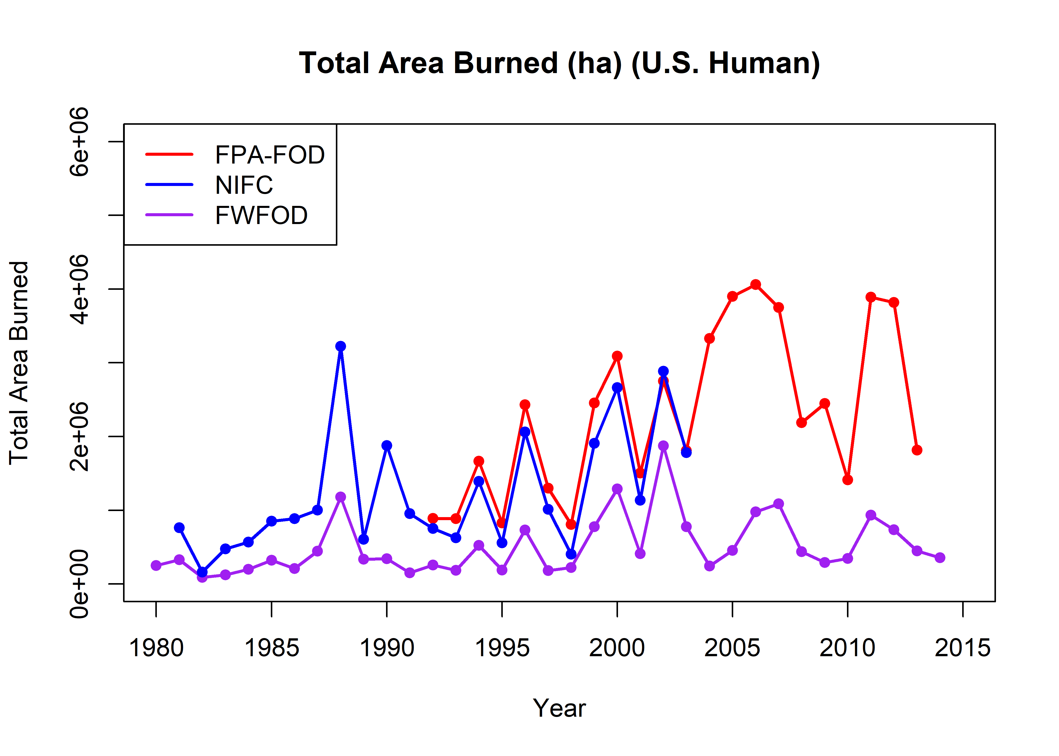
Scatter plots of the total areas burned in each data set:
oldpar <- par(mfrow=c(1,3))
plot(all_totalarea_hu$fpafod_hu_totalarea, all_totalarea_hu$nifc_hu_totalarea, xlim=c(0,6000000),
     ylim=c(0,6000000), pch=16, xlab="FPA-FOD", ylab="nifc_hu"); abline(0,1)
plot(all_totalarea_hu$fpafod_hu_totalarea, all_totalarea_hu$fwfod_hu_totalarea, xlim=c(0,6000000),
     ylim=c(0,6000000), pch=16, xlab="FPA-FOD", ylab="fwfod_hu",
     main="Total Area Burned (ha) (U.S. Human)"); abline(0,1)
plot(all_totalarea_hu$fwfod_hu_totalarea, all_totalarea_hu$nifc_hu_totalarea, xlim=c(0,6000000),
     ylim=c(0,6000000), pch=16, xlab="FWFOD", ylab="NIFC"); abline(0,1)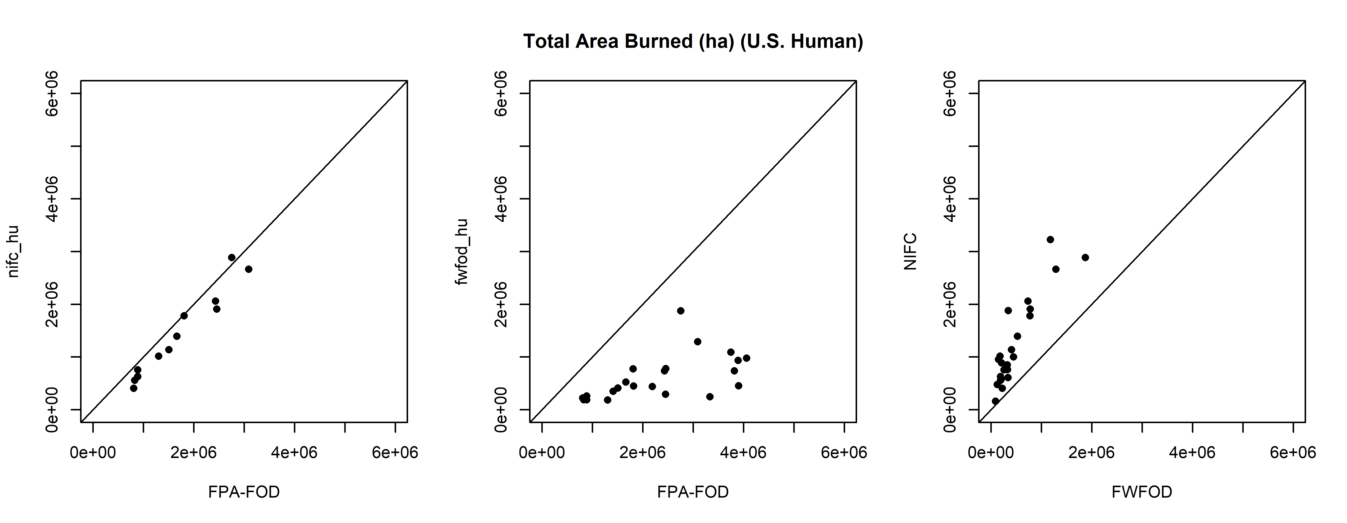
par(oldpar)5.2.3 Mean area burned
all_meanarea_hu <- data.frame(matrix(nrow = 36, ncol = 4))
names(all_meanarea_hu) <- c("Year", "fpafod_hu_meanarea", "nifc_hu_meanarea", "fwfod_hu_meanarea")
all_meanarea_hu["Year"] <- seq(1980, 2015, by=1)

fpafod_hu_mean_by_year <- tapply(fpafod_hu$AREA_HA, fpafod_hu$FIRE_YEAR, mean)
fpafod_hu_year <- as.numeric(unlist(dimnames(fpafod_hu_mean_by_year)))
fpafod_hu_mean_by_year <- as.numeric(fpafod_hu_mean_by_year)
all_meanarea_hu$fpafod_hu_meanarea[fpafod_hu_year-1980+1] <- fpafod_hu_mean_by_year

fwfod_hu_mean_by_year <- tapply(fwfod_hu$AREA, fwfod_hu$startyear, mean)
fwfod_hu_year <- as.numeric(unlist(dimnames(fwfod_hu_mean_by_year)))
fwfod_hu_mean_by_year <- as.numeric(fwfod_hu_mean_by_year)
all_meanarea_hu$fwfod_hu_meanarea[fwfod_hu_year-1980+1] <- fwfod_hu_mean_by_year

nifc_hu_size_year <- na.omit(cbind(nifc_hu$AREA,nifc_hu$YEAR))
nifc_hu_mean_by_year <- tapply(nifc_hu_size_year[,1],nifc_hu_size_year[,2], mean)
nifc_hu_year <- as.numeric(unlist(dimnames(nifc_hu_mean_by_year)))
nifc_hu_mean_by_year <- as.numeric(nifc_hu_mean_by_year)
all_meanarea_hu$nifc_hu_meanarea[nifc_hu_year-1980+1] <- nifc_hu_mean_by_year

all_meanarea_hu
## Year fpafod_hu_meanarea nifc_hu_meanarea fwfod_hu_meanarea
## 1 1980 NA NA 44.28053
## 2 1981 NA 160.80836 53.85396
## 3 1982 NA 53.24117 26.12257
## 4 1983 NA 114.24369 33.60840
## 5 1984 NA 104.96926 41.14954
## 6 1985 NA 116.86252 53.17169
## 7 1986 NA 52.31135 25.29974
## 8 1987 NA 47.73513 41.38159
## 9 1988 NA 153.00794 115.35638
## 10 1989 NA 31.68049 37.31438
## 11 1990 NA 95.72696 36.59427
## 12 1991 NA 51.55654 19.12410
## 13 1992 13.09469 35.51685 28.63310
## 14 1993 14.29323 39.17385 20.17180
## 15 1994 21.92913 53.82816 37.58846
## 16 1995 11.60197 30.32457 20.32030
## 17 1996 32.14969 93.94838 72.66416
## 18 1997 21.16718 67.38554 23.04818
## 19 1998 11.78585 22.72509 21.17537
## 20 1999 27.47142 92.07765 57.19483
## 21 2000 32.04353 115.18208 110.01748
## 22 2001 17.50134 52.60737 35.35426
## 23 2002 36.63227 140.89751 158.65799
## 24 2003 26.86357 90.31282 72.57760
## 25 2004 48.54992 NA 24.75057
## 26 2005 44.64507 NA 37.49714
## 27 2006 35.87688 NA 73.67100
## 28 2007 39.59393 NA 89.25566
## 29 2008 25.83633 NA 45.08941
## 30 2009 31.70590 NA 32.19674
## 31 2010 17.97961 NA 36.51709
## 32 2011 43.28778 NA 100.43850
## 33 2012 53.22947 NA 73.96045
## 34 2013 28.33779 NA 53.98083
## 35 2014 NA NA 39.72876
## 36 2015 NA NA NAplot(fpafod_hu_mean_by_year ~ fpafod_hu_year, type="o", col="red", pch=16, lwd=2, xlim=c(1980,2015),
ylim=c(0,300), xlab="Year", ylab="Mean Area Burned",
main="Mean Area Burned (ha) (U.S. Human)")
points(fwfod_hu_mean_by_year ~ fwfod_hu_year, type="o", col="purple", pch=16, lwd=2)
points(nifc_hu_mean_by_year ~ nifc_hu_year, type="o", col="blue", pch=16, lwd=2)
legend("topleft", legend=c("FPA-FOD","NIFC","FWFOD"), lwd=2, col=c("red","blue","purple"))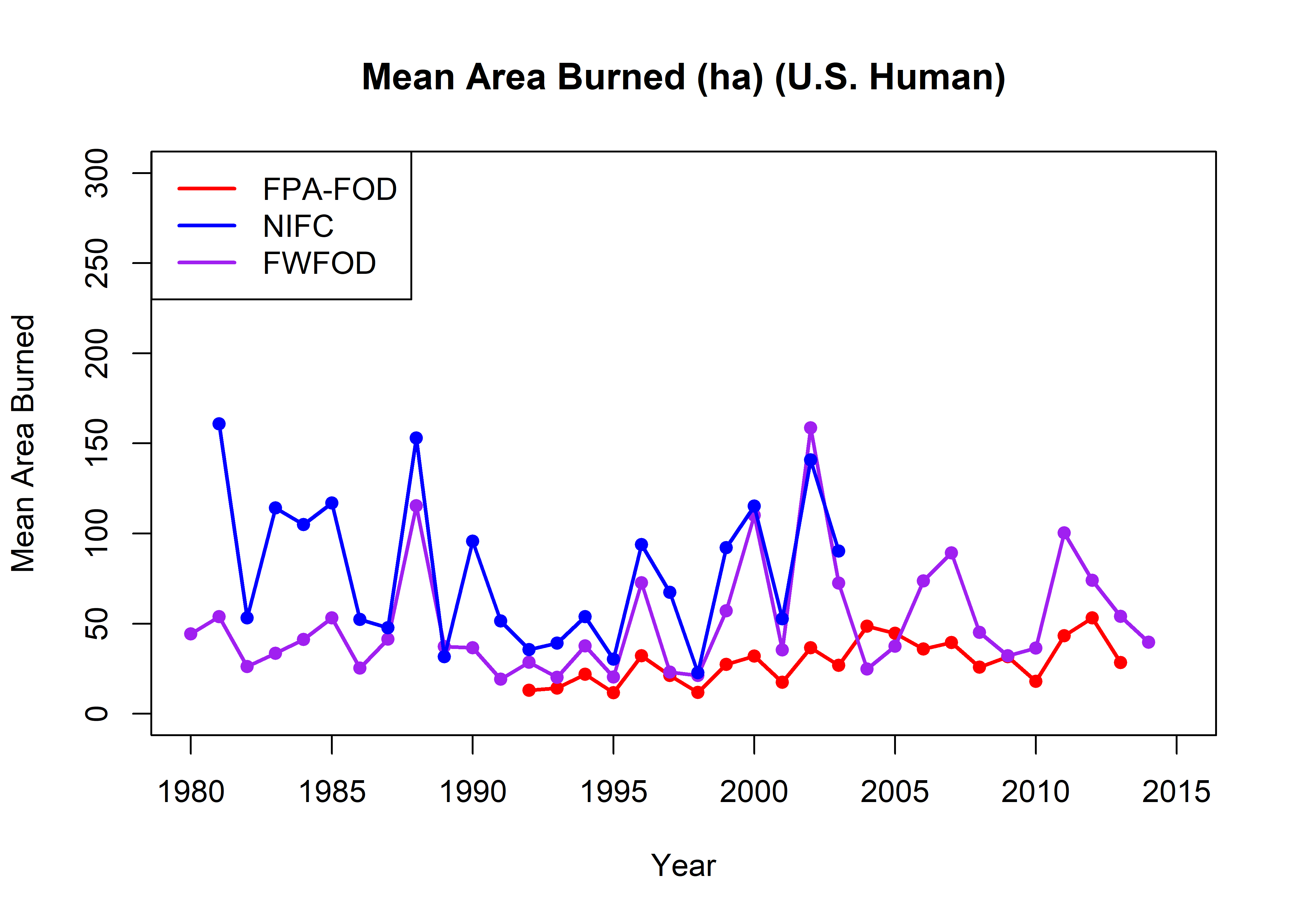
Scatter plots of the mean areas burned in each data set:
oldpar <- par(mfrow=c(1,3))
plot(all_meanarea_hu$fpafod_hu_meanarea, all_meanarea_hu$nifc_hu_meanarea, xlim=c(0,300),
     ylim=c(0,300), pch=16, xlab="FPA-FOD", ylab="NIFC"); abline(0,1)
plot(all_meanarea_hu$fpafod_hu_meanarea, all_meanarea_hu$fwfod_hu_meanarea, xlim=c(0,300),
     ylim=c(0,300), pch=16, xlab="FPA-FOD", ylab="FWFOD",
     main="Mean Area Burned (ha) (U.S. All"); abline(0,1)
plot(all_meanarea_hu$fwfod_hu_meanarea, all_meanarea_hu$nifc_hu_meanarea, xlim=c(0,300),
     ylim=c(0,300 ), pch=16, xlab="FWFOD", ylab="NIFC"); abline(0,1)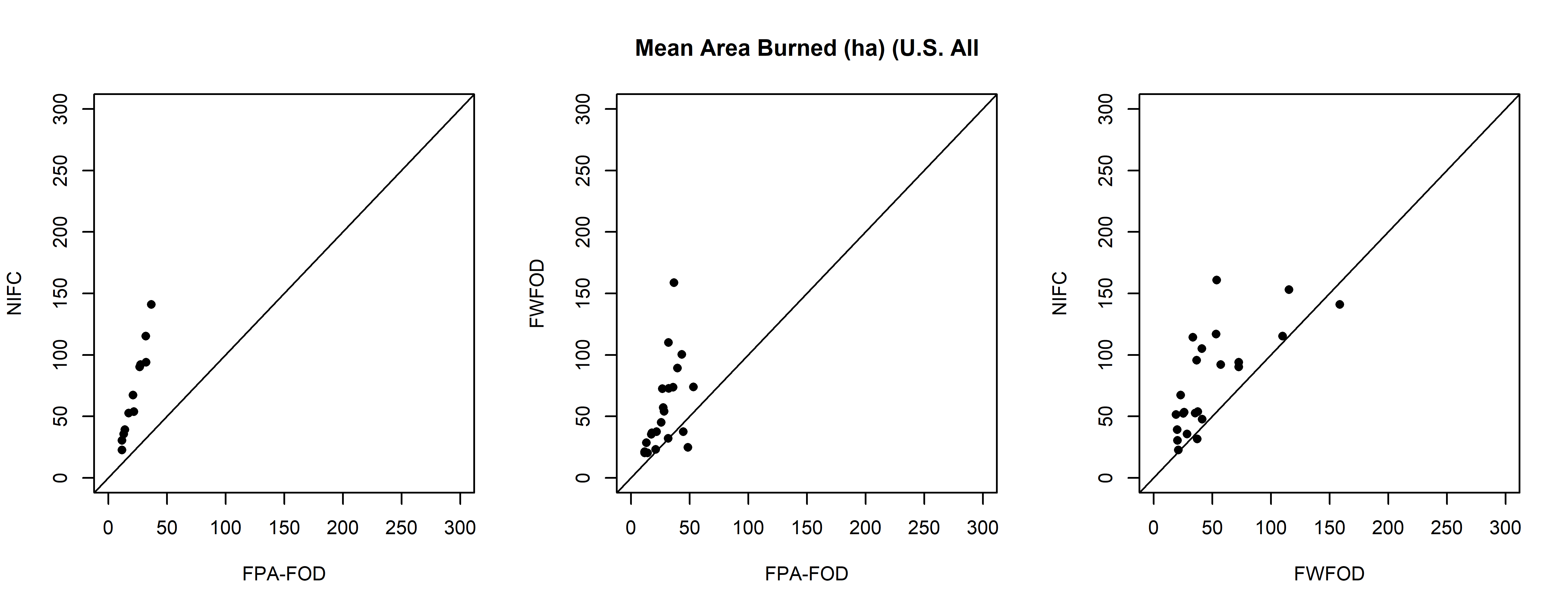
par(oldpar)5.3 Fire size class by year
sizecuts <- c(0.0,0.01,0.1,1,10,100,1000,10000) # c(0.0,0.00001,10,1000000) #
fpafod_hu$sizeclass <- cut(fpafod_hu$AREA_HA,sizecuts)
table(fpafod_hu$sizeclass)
##
## (0,0.01] (0.01,0.1] (0.1,1] (1,10] (10,100] (100,1e+03] (1e+03,1e+04]
## 31743 520703 655620 378638 114084 21048 4777fpafod.tablesize <- table(fpafod_hu$FIRE_YEAR, fpafod_hu$sizeclass)
mosaicplot(fpafod.tablesize, color=TRUE, cex.axis=0.6, las=2, main="FPA-FOD by size, Human Fires")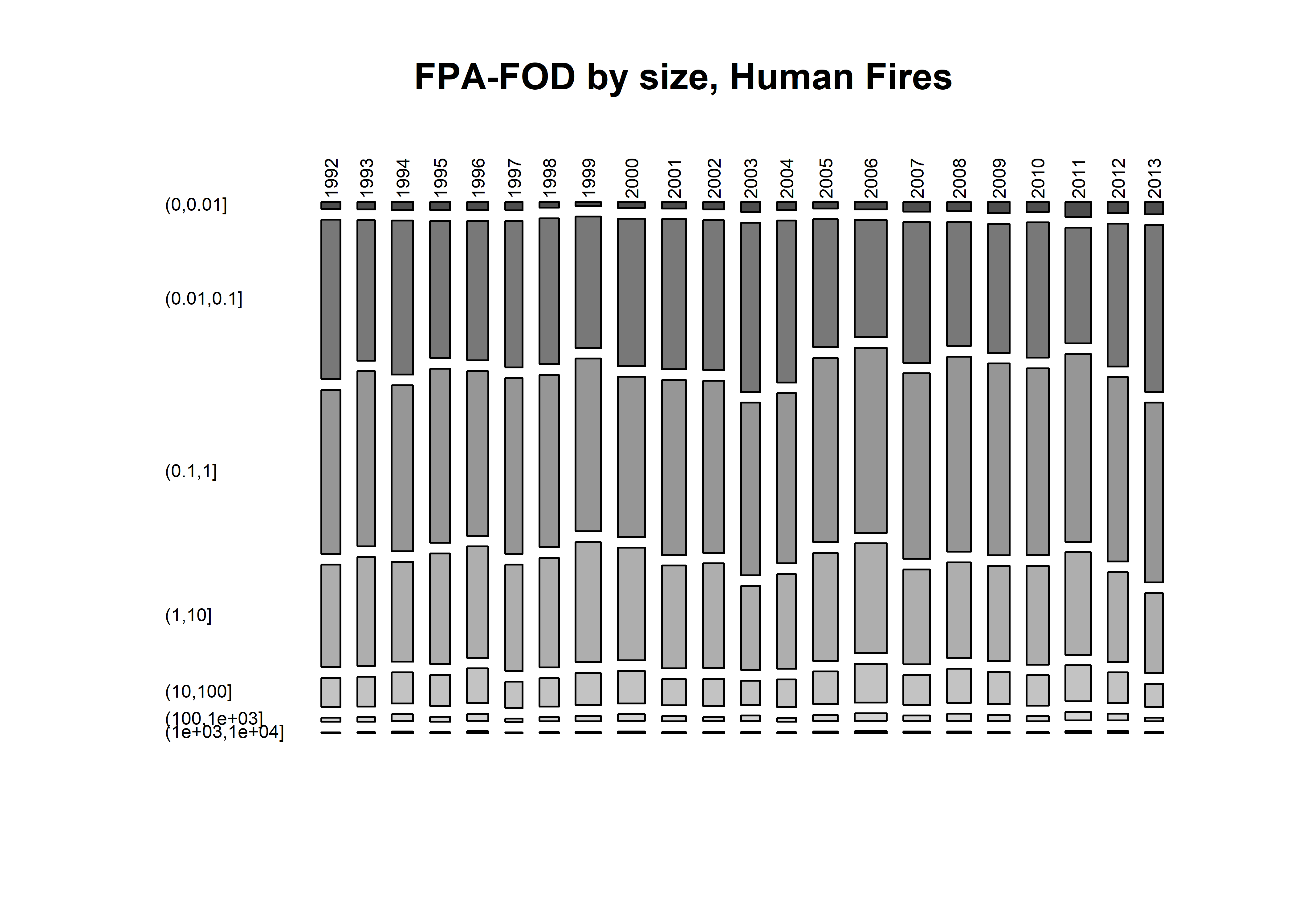
nifc_hu$sizeclass <- cut(nifc_hu$AREA,sizecuts)
table(nifc_hu$sizeclass)
##
## (0,0.01] (0.01,0.1] (0.1,1] (1,10] (10,100] (100,1e+03] (1e+03,1e+04]
## 0 190687 94969 50546 23905 9287 3069nifc.tablesize <- table(nifc_hu$YEAR, nifc_hu$sizeclass)
mosaicplot(nifc.tablesize, color=TRUE, cex.axis=0.6, las=2, main="NIFC by size, Human Fires")
fwfod_hu$sizeclass <- cut(fwfod_hu$AREA,sizecuts)
table(fwfod_hu$sizeclass)
##
## (0,0.01] (0.01,0.1] (0.1,1] (1,10] (10,100] (100,1e+03] (1e+03,1e+04]
## 1621 141189 90990 53350 24994 7413 1772fwfod.tablesize <- table(fwfod_hu$startyear, fwfod_hu$sizeclass)
mosaicplot(fwfod.tablesize, color=TRUE, cex.axis=0.6, las=2, main="FWFOD by size, Human Fires")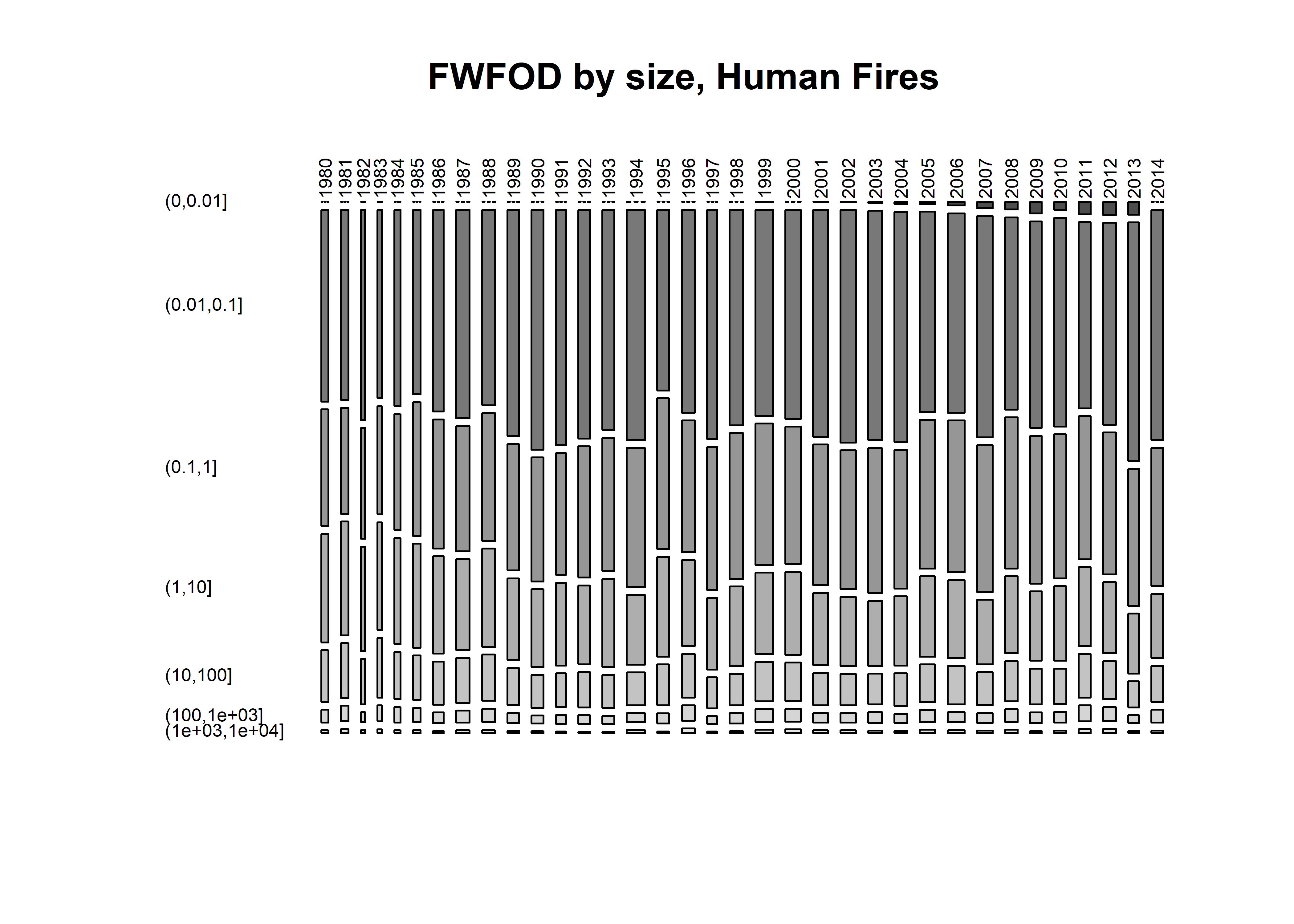
5.4 Fire areas by database
lt_fpafod <- cbind(fpafod_hu$FIRE_YEAR, fpafod_hu$AREA_HA, "FPA-FOD")
lt_nifc <- cbind(nifc_hu$YEAR, nifc_hu$AREA, "NIFC")
lt_fwfod <- cbind(fwfod_hu$startyear, fwfod_hu$AREA, "FWFOD")
lt_fires <-as.data.frame(rbind(lt_fpafod,lt_nifc,lt_fwfod))
#str(lt_fires)
names(lt_fires) <- c("Year","AreaHA", "db")
#summary(lt_fires)
lt_fires[,1] <- as.integer(as.character(lt_fires[,1]))
lt_fires[,2] <- as.numeric(as.character(lt_fires[,2]))
#summary(lt_fires)
lt_fires <- na.omit(lt_fires)

sizecuts <- c(0.0,0.00001,10,1000000) #
lt_fires$sizeclass <- cut(lt_fires$AreaHA,sizecuts)
table(lt_fires$sizeclass)
##
## (0,1e-05] (1e-05,10] (10,1e+06]
## 1 2210045 211997lt_tablesize <- table(lt_fires$db, lt_fires$sizeclass)
mosaicplot(lt_tablesize, color=TRUE, cex.axis=0.6, las=2, main="Human Fires -- Size (ha) by Database")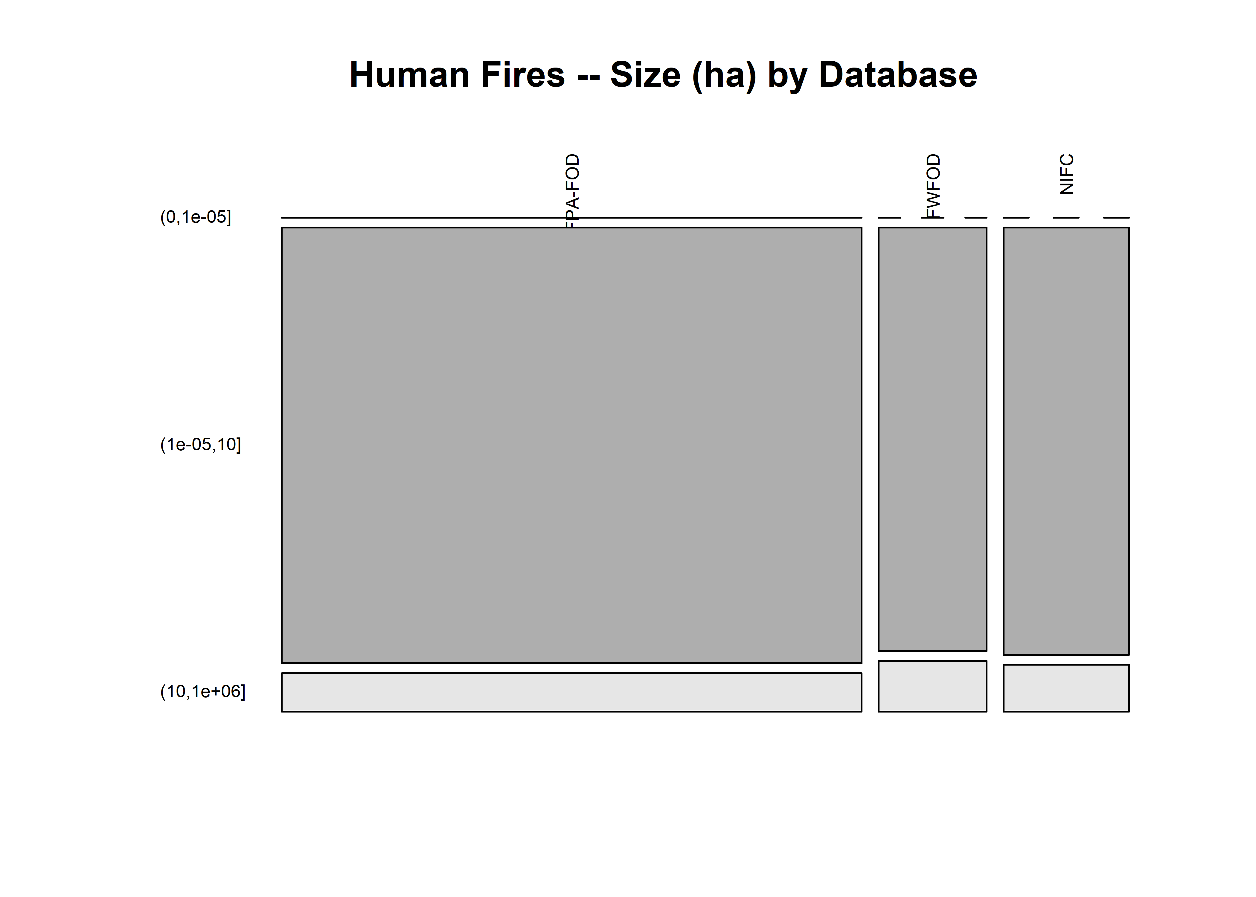
sizecuts <- c(0.0,0.01,0.1,1,10,100,1000,10000) # c(0.0,0.00001,10,1000000) #
lt_fires$sizeclass <- cut(lt_fires$AreaHA,sizecuts)
table(lt_fires$sizeclass)
##
## (0,0.01] (0.01,0.1] (0.1,1] (1,10] (10,100] (100,1e+03] (1e+03,1e+04]
## 33364 852574 841576 482532 162980 37747 9617lt_tablesize <- table(lt_fires$db, lt_fires$sizeclass)
mosaicplot(lt_tablesize, color=TRUE, cex.axis=0.6, las=2, main="Human Fires -- Size (ha) by Database")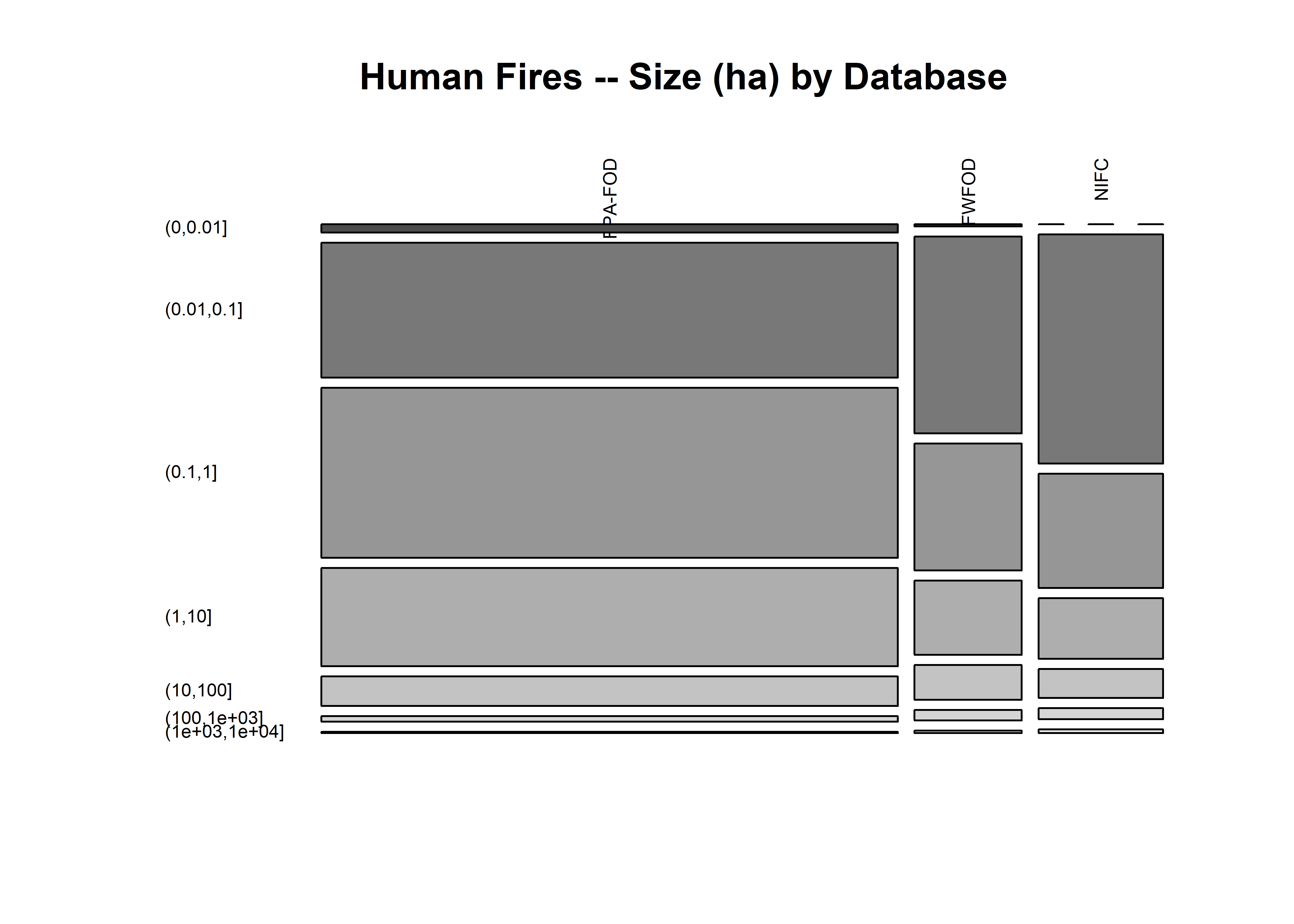
5.5 Fire frequency by month and year
fpafod.tablemon <- table(fpafod_hu$FIRE_YEAR,
  fpafod_hu$startmon)
mosaicplot(fpafod.tablemon, color=monthcolors, cex.axis=0.6, las=3, main="fpafod, Human Fires, All Agencies")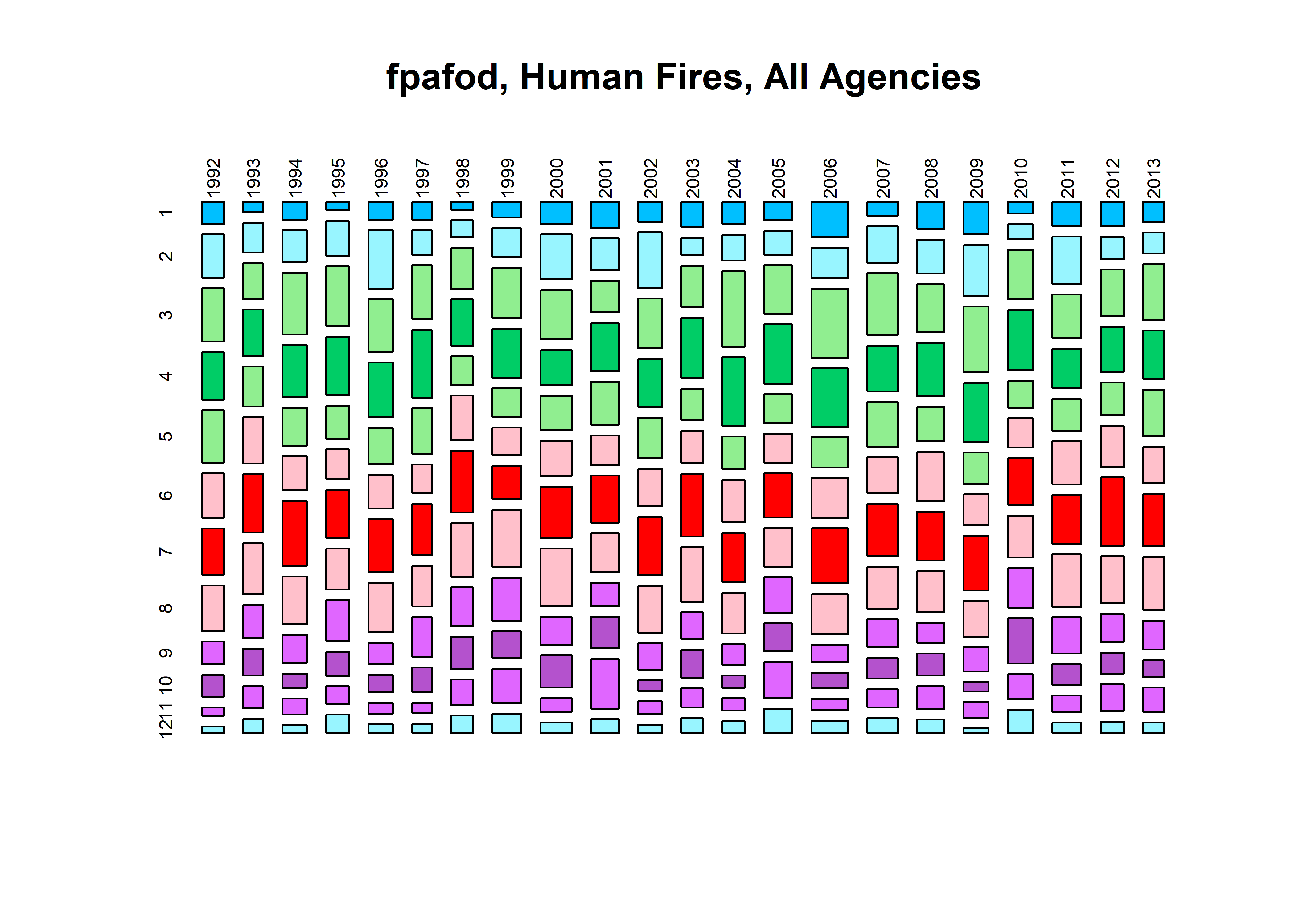
nifc.tablemon <- table(nifc_hu$YEAR, nifc_hu$startmon)
mosaicplot(nifc.tablemon, color=monthcolors, cex.axis=0.6, las=3, main="nifc, Human Fires, All Agencies")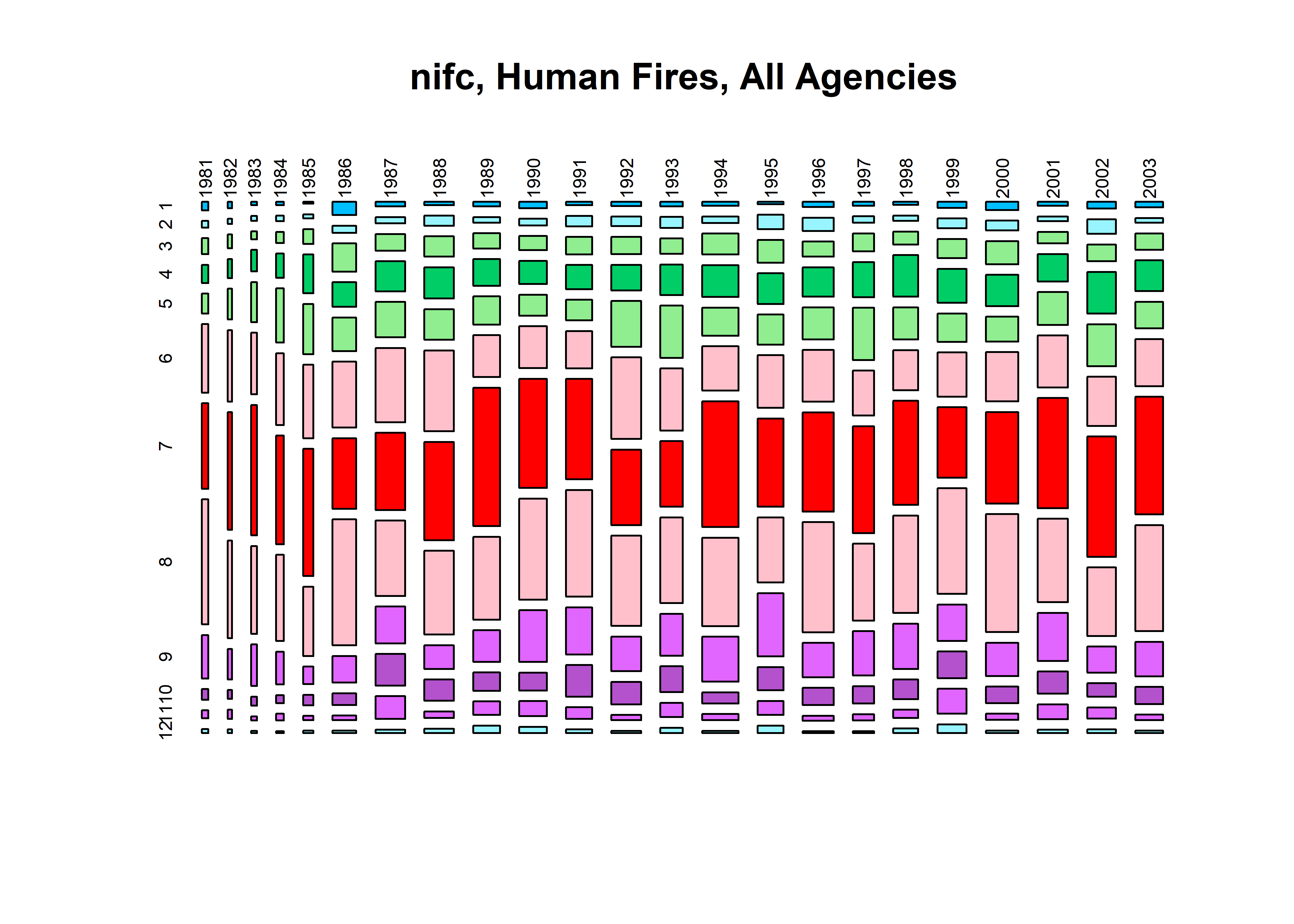
fwfod.tablemon <- table(fwfod_hu$startyear, fwfod_hu$startmon)
mosaicplot(fwfod.tablemon, color=monthcolors, cex.axis=0.6, las=3, main="fwfod, Human Fires, All Agencies")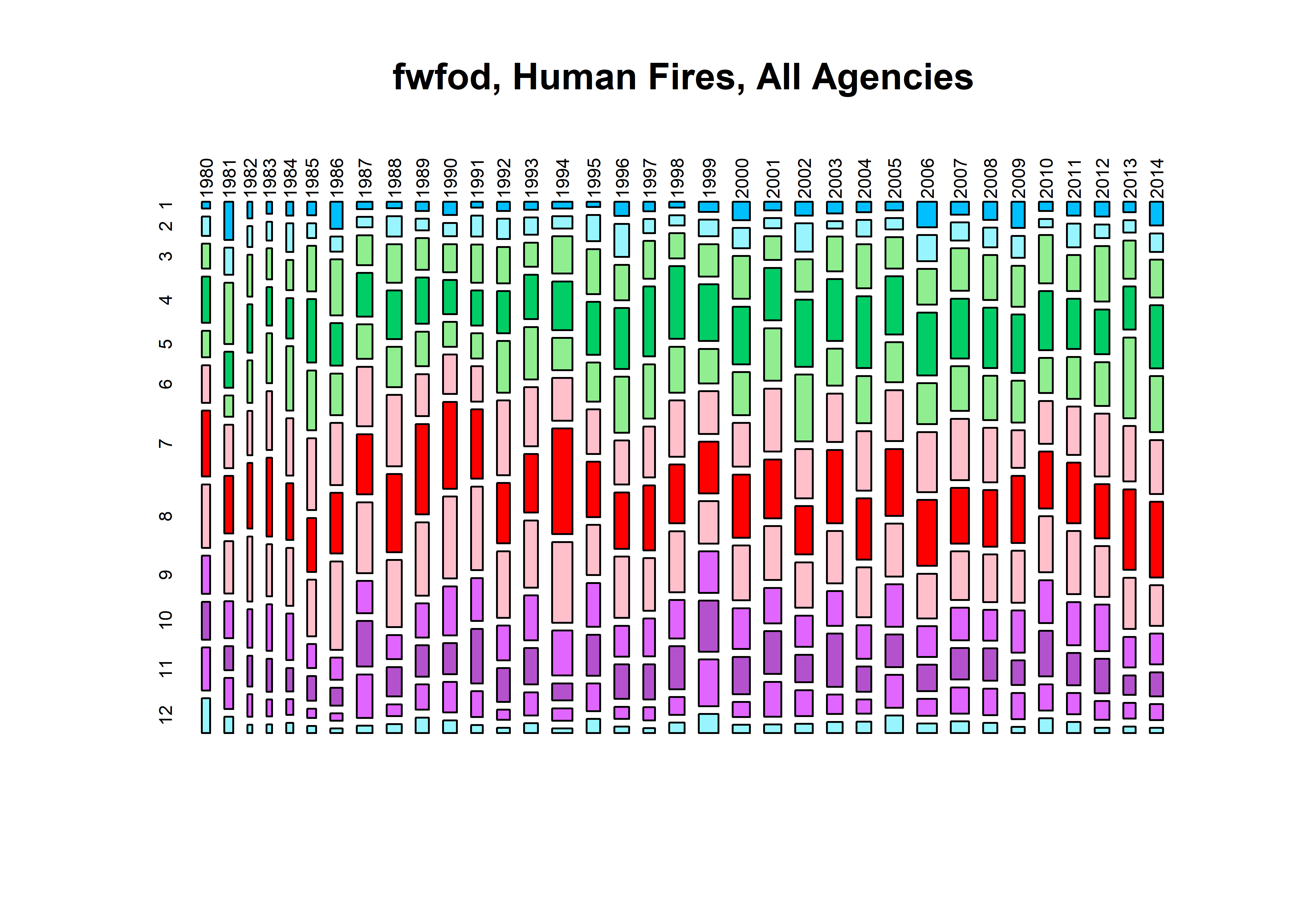
5.6 U.S. Forest Service
table(fpafod_hu$FIRE_YEAR[fpafod_hu$NWCG_REPORTING_AGENCY =="FS"])##
## 1992 1993 1994 1995 1996 1997 1998 1999 2000 2001 2002 2003 2004 2005 2006 2007 2008
## 11471 7731 14532 9231 11522 7913 9433 10994 11890 11018 9554 10727 8660 7661 10992 8960 7400
## 2009 2010 2011 2012 2013
## 7845 6951 7283 7518 7445table(nifc_hu$YEAR[nifc_hu$AGENCY_COD=="USFS"])##
## 1981 1982 1983 1984 1985 1986 1987 1988 1989 1990 1991 1992 1993 1994 1995 1996 1997
## 5 1 77 123 70 10604 13436 12718 11861 11875 10893 11649 7825 14751 9301 11580 7945
## 1998 1999 2000 2001 2002 2003
## 9471 11024 11983 11099 9538 10608table(fwfod_hu$startyear[fwfod_hu$ORGANIZATI=="FS"])##
## 1980 1981 1982 1983 1984 1985 1986 1987 1988 1989 1990 1991 1992 1993 1994 1995 1996 1997 1998 1999 2000
## 4165 4281 2148 1976 2503 2882 5643 7391 6536 5604 5985 4284 4382 4556 8731 3818 4980 3935 4497 6120 5113
## 2001 2002 2003 2004 2005 2006 2007 2008 2009 2010 2011 2012 2013 2014
## 5128 4406 3898 3705 4147 4615 4298 3743 3932 4157 3726 4023 3092 3037fpafod.tablemon <- table(fpafod_hu$FIRE_YEAR[fpafod_hu$NWCG_REPORTING_AGENCY == "FS" &
fpafod_hu$STAT_CAUSE_CODE == 1], fpafod_hu$startmon[fpafod_hu$NWCG_REPORTING_AGENCY == "FS" &
fpafod_hu$STAT_CAUSE_CODE == 1])
mosaicplot(fpafod.tablemon, color=monthcolors, cex.axis=0.6, las=3, main="fpafod, Human Fires, FS")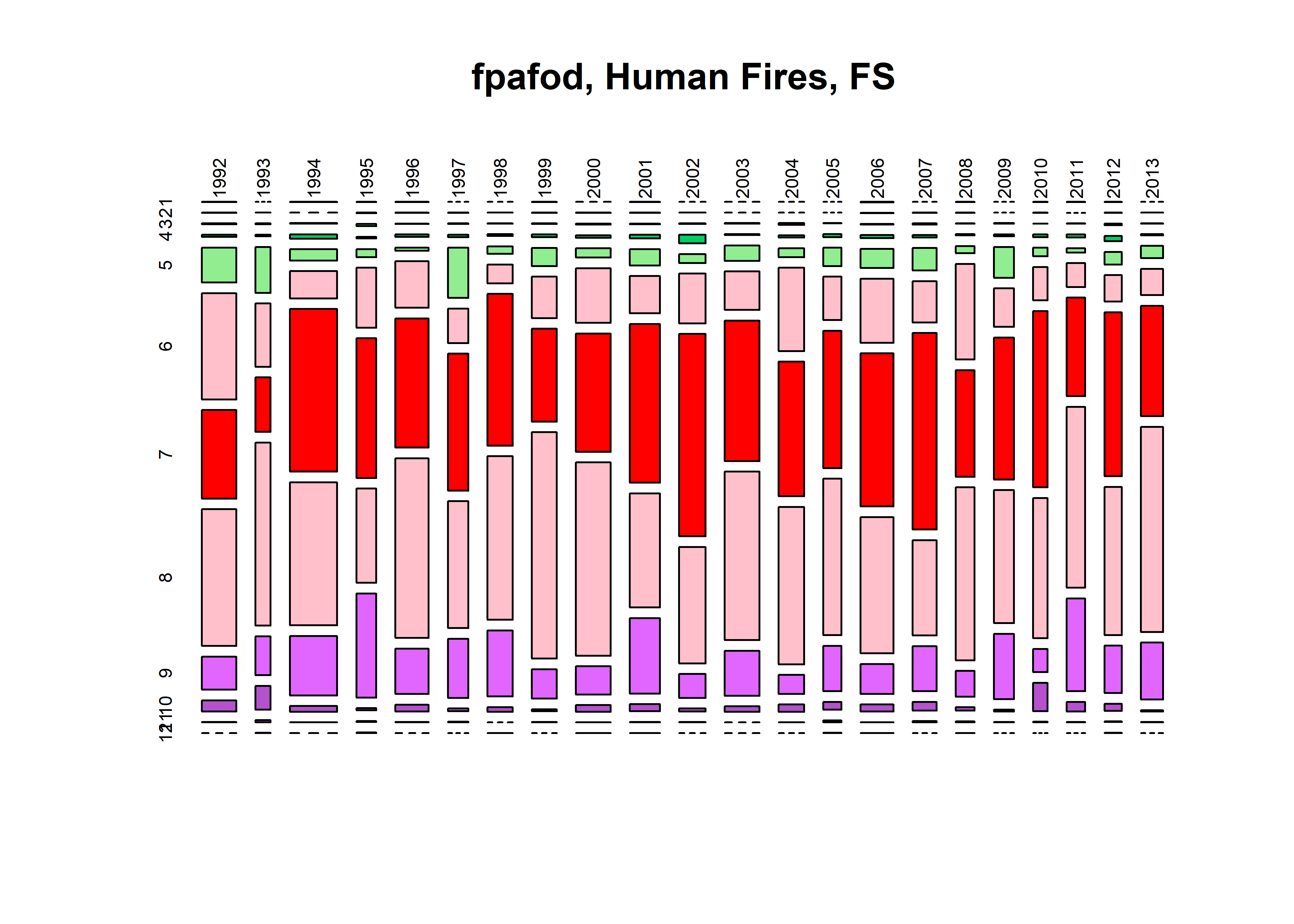
nifc.tablemon <- table(nifc_hu$YEAR[nifc_hu$AGENCY_COD== "USFS"],
  nifc_hu$startmon[nifc_hu$AGENCY_COD== "USFS"])
mosaicplot(nifc.tablemon, color=monthcolors, cex.axis=0.6, las=3, main="nifc, Human Fires, FS")
fwfod.tablemon <- table(fwfod_hu$startyear[fwfod_hu$ORGANIZATI== "FS"],
  fwfod_hu$startmon[fwfod_hu$ORGANIZATI== "FS"])
mosaicplot(fwfod.tablemon, color=monthcolors, cex.axis=0.6, las=3, main="fwfod, Human Fires, FS")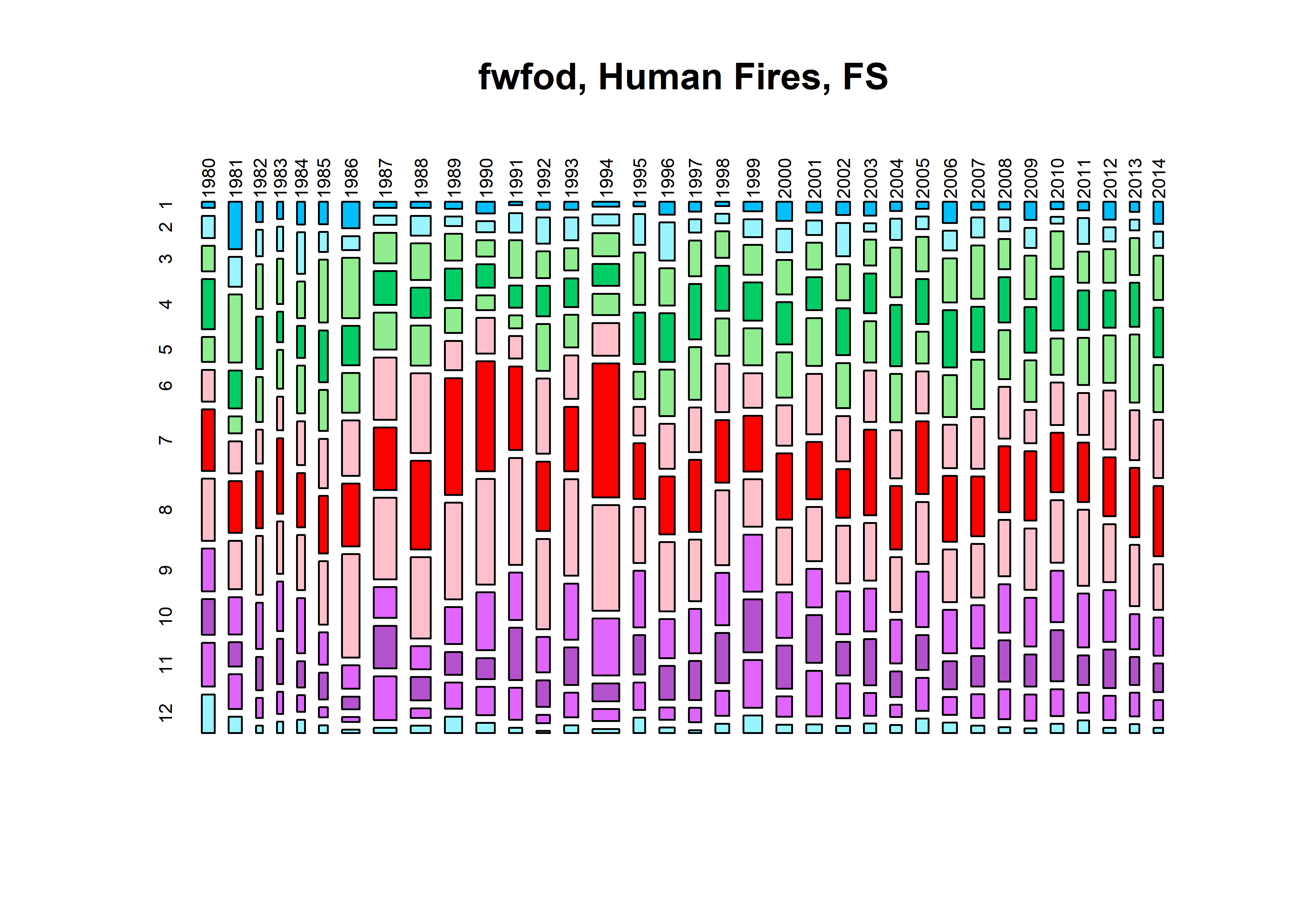
hist(nifc_hu$YEAR, xlim=c(1980,2015), ylim=c(0,30000),
   breaks=seq(1979.5,2014.5,by=1), col="lightblue", border="blue", main="Human Fires")
hist(fpafod_hu$FIRE_YEAR, xlim=c(1980,2015), ylim=c(0,120000),
  breaks=seq(1979.5,2014.5,by=1), xlab="Year", col="pink", border="red", add=TRUE)
hist(fwfod_hu$startyear, xlim=c(1980,2015), ylim=c(0,120000),
  breaks=seq(1979.5,2014.5,by=1), add=TRUE,  border="purple")
hist(nifc_hu$YEAR, xlim=c(1980,2015), ylim=c(0,120000),
   breaks=seq(1979.5,2014.5,by=1), border="blue", add=TRUE)
legend("topleft", legend=c("FPA-FOD","NIFC","FWFOD"), lwd=2, col=c("red","blue","purple"))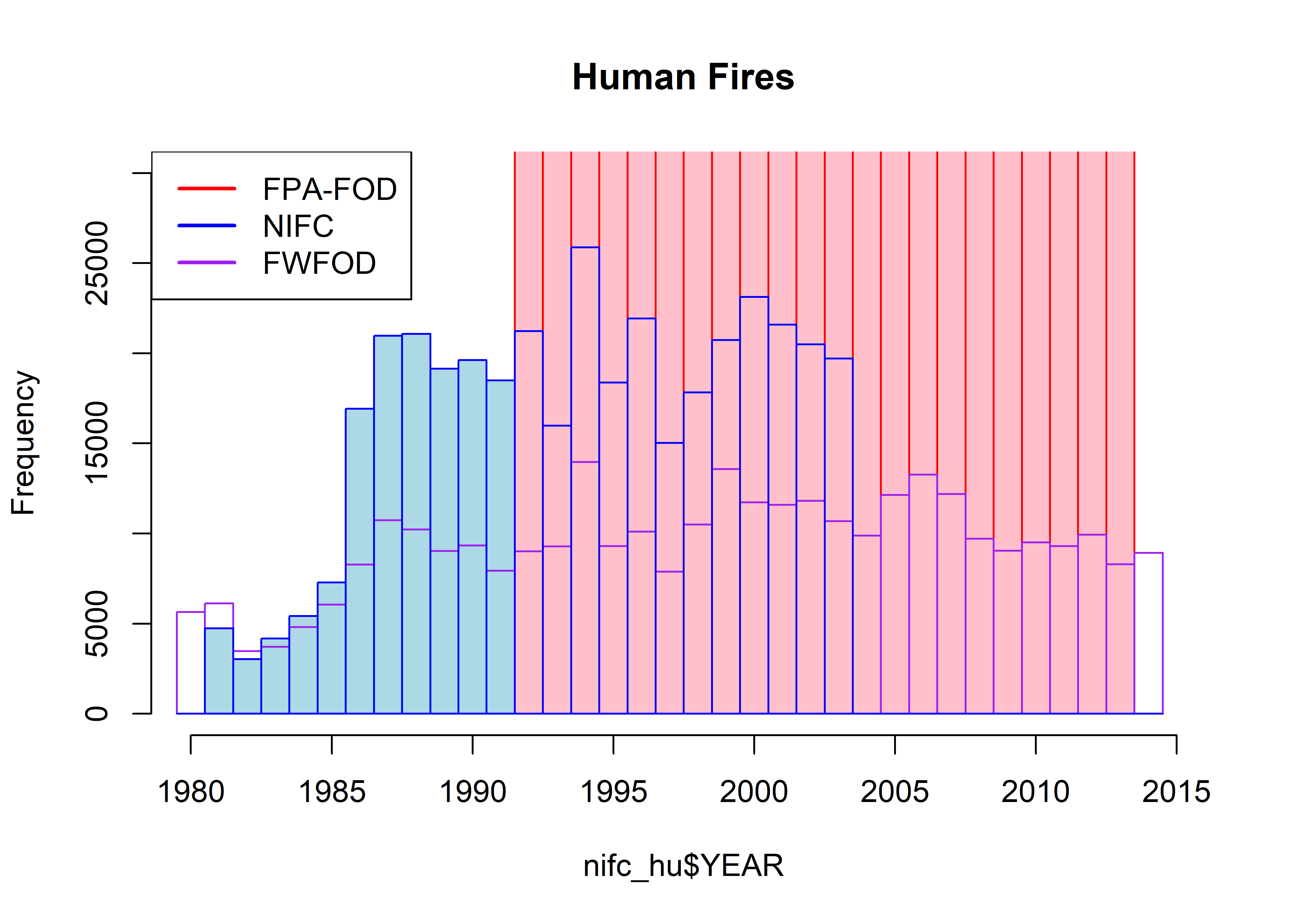
hist(nifc_hu$YEAR[nifc_hu$AGENCY_COD=="USFS"], xlim=c(1980,2015), ylim=c(0,15000),
   breaks=seq(1979.5,2014.5,by=1), col="lightblue", border="blue", main="Human Fires, USFS")
hist(fpafod_hu$FIRE_YEAR[fpafod_hu$NWCG_REPORTING_AGENCY =="FS"],
  xlim=c(1980,2015), ylim=c(0,120000), breaks=seq(1979.5,2014.5,by=1), xlab="Year", col="pink",
  border="red", add=TRUE)
hist(fwfod_hu$startyear[fwfod_hu$ORGANIZATI=="FS"], xlim=c(1980,2015), ylim=c(0,120000),
  breaks=seq(1979.5,2014.5,by=1), add=TRUE, border="purple")
hist(nifc_hu$YEAR[nifc_hu$AGENCY_COD=="USFS"], xlim=c(1980,2015), ylim=c(0,120000),
   breaks=seq(1979.5,2014.5,by=1), border="blue", add=TRUE)
legend("topleft", legend=c("FPA-FOD","NIFC","FWFOD"), lwd=2, col=c("red","blue","purple"))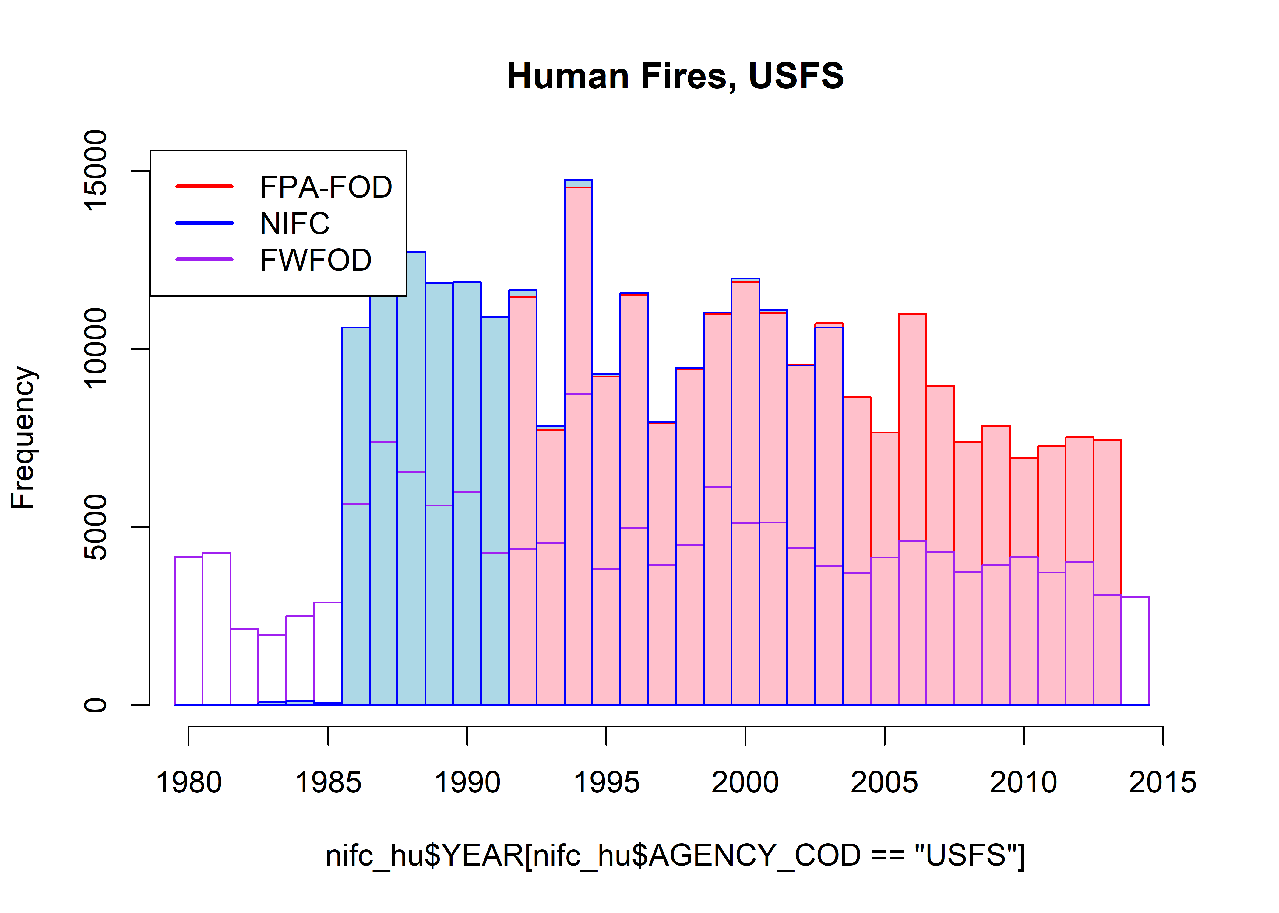
6 Correlations among time series
The correlations bewteen the different annual time series can be examined to determine for fire type (all, lightning (lt) and human (hu)) and statistic (number, total area, mean area), which data sets are more highly correlated with one another.
cor_all <- cor(cbind(all_num[2:4], all_totalarea[2:4], all_meanarea[2:4]),
  use="pairwise.complete.obs")
cor_all
## fpafod_num nifc_num fwfod_num fpafod_totalarea nifc_totalarea fwfod_totalarea
## fpafod_num 1.0000000 0.6367649 0.53775271 0.6506131 0.6049896 0.4146442
## nifc_num 0.6367649 1.0000000 0.96265195 0.4860339 0.5577238 0.4984224
## fwfod_num 0.5377527 0.9626519 1.00000000 0.2988121 0.6403894 0.5592743
## fpafod_totalarea 0.6506131 0.4860339 0.29881205 1.0000000 0.9780410 0.8380113
## nifc_totalarea 0.6049896 0.5577238 0.64038944 0.9780410 1.0000000 0.9801698
## fwfod_totalarea 0.4146442 0.4984224 0.55927431 0.8380113 0.9801698 1.0000000
## fpafod_meanarea 0.3433833 0.3665485 0.14198698 0.9313070 0.9728766 0.8454758
## nifc_meanarea 0.4888972 -0.1793197 -0.02932397 0.9373432 0.6720063 0.6834516
## fwfod_meanarea 0.2897016 0.2722471 0.36225340 0.8228616 0.9238413 0.9656798
## fpafod_meanarea nifc_meanarea fwfod_meanarea
## fpafod_num 0.3433833 0.48889724 0.2897016
## nifc_num 0.3665485 -0.17931967 0.2722471
## fwfod_num 0.1419870 -0.02932397 0.3622534
## fpafod_totalarea 0.9313070 0.93734323 0.8228616
## nifc_totalarea 0.9728766 0.67200630 0.9238413
## fwfod_totalarea 0.8454758 0.68345160 0.9656798
## fpafod_meanarea 1.0000000 0.97029774 0.8843532
## nifc_meanarea 0.9702977 1.00000000 0.8231916
## fwfod_meanarea 0.8843532 0.82319159 1.0000000cor_lt <- cor(cbind(all_num_lt[2:4], all_totalarea_lt[2:4], all_meanarea_lt[2:4]),
use="pairwise.complete.obs")
cor_lt## fpafod_lt_num nifc_lt_num fwfod_lt_num fpafod_lt_totalarea nifc_lt_totalarea
## fpafod_lt_num 1.00000000 0.95193812 0.8271399 0.3244636 0.6009423
## nifc_lt_num 0.95193812 1.00000000 0.9490102 0.4449422 0.5974468
## fwfod_lt_num 0.82713986 0.94901016 1.0000000 0.1412459 0.6047574
## fpafod_lt_totalarea 0.32446358 0.44494217 0.1412459 1.0000000 0.9805042
## nifc_lt_totalarea 0.60094232 0.59744678 0.6047574 0.9805042 1.0000000
## fwfod_lt_totalarea 0.17287468 0.50639428 0.3827925 0.9111658 0.9564264
## fpafod_lt_meanarea 0.04087153 0.09228316 -0.1064310 0.9520666 0.8682430
## nifc_lt_meanarea 0.24981644 -0.21123377 -0.1731203 0.9031614 0.5880497
## fwfod_lt_meanarea -0.04345749 0.20983878 0.1425409 0.8561208 0.8519219
## fwfod_lt_totalarea fpafod_lt_meanarea nifc_lt_meanarea fwfod_lt_meanarea
## fpafod_lt_num 0.1728747 0.04087153 0.2498164 -0.04345749
## nifc_lt_num 0.5063943 0.09228316 -0.2112338 0.20983878
## fwfod_lt_num 0.3827925 -0.10643101 -0.1731203 0.14254095
## fpafod_lt_totalarea 0.9111658 0.95206663 0.9031614 0.85612076
## nifc_lt_totalarea 0.9564264 0.86824299 0.5880497 0.85192187
## fwfod_lt_totalarea 1.0000000 0.91226842 0.5871530 0.95326837
## fpafod_lt_meanarea 0.9122684 1.00000000 0.9661934 0.93136586
## nifc_lt_meanarea 0.5871530 0.96619344 1.0000000 0.78337580
## fwfod_lt_meanarea 0.9532684 0.93136586 0.7833758 1.00000000cor_hu <- cor(cbind(all_num_hu[2:4], all_totalarea_hu[2:4], all_meanarea_hu[2:4]),
use="pairwise.complete.obs")
cor_hu## fpafod_hu_num nifc_hu_num fwfod_hu_num fpafod_hu_totalarea nifc_hu_totalarea
## fpafod_hu_num 1.0000000 0.6494852 0.6448639 0.6506131 0.5897754
## nifc_hu_num 0.6494852 1.0000000 0.9152231 0.5150944 0.5604544
## fwfod_hu_num 0.6448639 0.9152231 1.0000000 0.3824939 0.5870342
## fpafod_hu_totalarea 0.6506131 0.5150944 0.3824939 1.0000000 0.9746780
## nifc_hu_totalarea 0.5897754 0.5604544 0.5870342 0.9746780 1.0000000
## fwfod_hu_totalarea 0.4995281 0.4648918 0.5780915 0.5672776 0.8999157
## fpafod_hu_meanarea 0.3433833 0.3984748 0.1927982 0.9313070 0.9744876
## nifc_hu_meanarea 0.4682426 -0.2734630 -0.1301930 0.9353397 0.5896878
## fwfod_hu_meanarea 0.4142673 0.2628858 0.3523661 0.5633570 0.8632554
## fwfod_hu_totalarea fpafod_hu_meanarea nifc_hu_meanarea fwfod_hu_meanarea
## fpafod_hu_num 0.4995281 0.3433833 0.4682426 0.4142673
## nifc_hu_num 0.4648918 0.3984748 -0.2734630 0.2628858
## fwfod_hu_num 0.5780915 0.1927982 -0.1301930 0.3523661
## fpafod_hu_totalarea 0.5672776 0.9313070 0.9353397 0.5633570
## nifc_hu_totalarea 0.8999157 0.9744876 0.5896878 0.8632554
## fwfod_hu_totalarea 1.0000000 0.4738618 0.5627374 0.9598189
## fpafod_hu_meanarea 0.4738618 1.0000000 0.9757680 0.5066698
## nifc_hu_meanarea 0.5627374 0.9757680 1.0000000 0.7144638
## fwfod_hu_meanarea 0.9598189 0.5066698 0.7144638 1.0000000The strength of the correlations can be conveniently examined using the following correlation plots, by focusing on the 3x3 groups of cells along the main diagonal of the plots. Each of these 3x3 groups shows variations in correlations among the different data sets for a particular variable (i.e. number, total area, mean area):
library(corrplot)
oldpar <- par(mfrow=c(1,2))
corrplot(cor_all, method="shade", tl.cex=0.5, tl.col = "black", cl.cex=0.5)
  title(main = "All U.S. Data", cex.main=1)
par(oldpar); oldpar <- par(mfrow=c(1,2))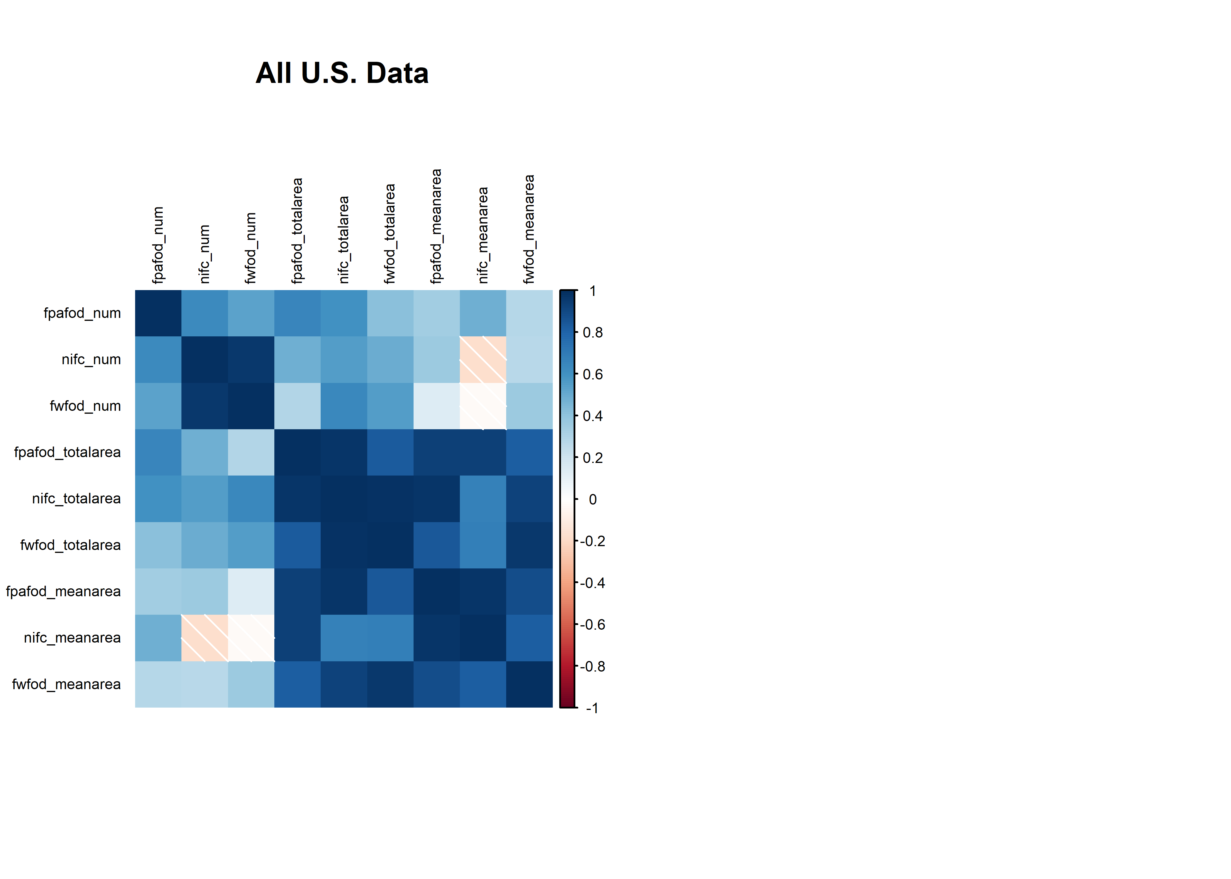
corrplot(cor_lt, method="shade", tl.cex=0.5, tl.col = "black", cl.cex=0.5)
  title(main = "Lightning Only", cex.main=1)
corrplot(cor_hu, method="shade", tl.cex=0.5, tl.col = "black", cl.cex=0.5)
  title(main = "Human Only", cex.main=1)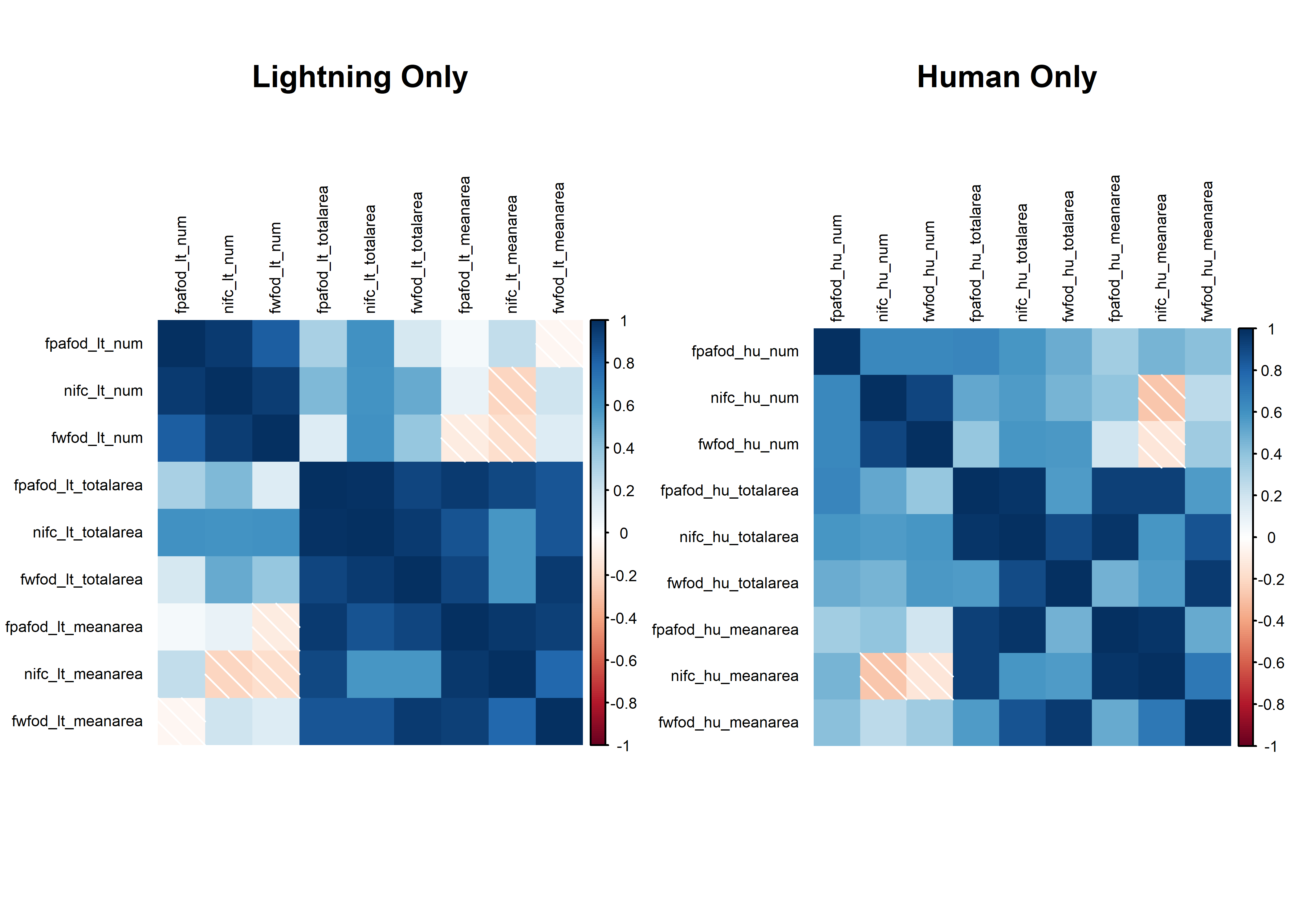
par(oldpar)In comparing the data sets, there are two things to focus on: 1) bias, or over- or under-representation of fires in one data set or another, and 2) interannual variations and the strength of the correlations among series. One overarching observation that can be made is that there are many more fires in general, and human-started fires in particular, in the FPA-FOD data set than in the NIFC or FWFOD data sets, and those additional fires are generally small. Other observations include:
All fires:
- The much larger number of fires in the FPA-FOD data set makes it difficult to compare the different data sets. If the FPA-FOD data are regarded as definitive, the NIFC and FWFOD data sets are greatly biased downward.
- Where the series overlap, the NIFC total area burned data are better correlated with the FPA-FOD data than are the FWFOD data, although for mean area burned, both the NIFC and FWFOD data have a large positive bias, related to the large number of fires in the 0.1 - 1 ha size range in the FPA-FOD data.
Lightning-started fires:
- For lightning-started fires, the individual annual time series are much better correlated than those for all fires, but there is still a noticeable negative bias in total number of fires and and postitive bias in mean fire area for the NIFC and FWFOD data relative to the FPA-FOD.
- Two years in the FWFOD data set, 2004 and 2005, seem to have anomalously large total areas burned relative to the FPA-FOD data. Otherwise, the series are well correlated.
Human-started fires:
- The number of human-started fires is quite different across the data set with the FPA-FOD data set recording the most fires, and the NIFC data set the least. In contrast, interannual variations among the series is reasonably well correlated.
- For annual total area burned, the FPA-FOD and NIFC records are fairly well correlated, while the FWFOD record is not well correlated with either, and also appears to be systematically lower.
- For mean area burned by human-started fires, as for all fires the FPA-FOD the NIFC and FWFOD data have a large positive bias, related to the large number of fires in the FPA-FOD data. The interannual variations of the FPA-FOD and NIFC data are again highly correlated.
Overall, the annual values NIFC total area burned and mean area burned data are better correlated with the FPA-FOD across all, lightning-started and human-started fires and show similar or lower biases relative to the FPA-FOD data than do the FWFOD data. In the case of numbers of fires across all fire types, the NIFC and FWFOD are roughly similar in their correlation with or bias relative to the FPA-FOD data.
7 Summary
Overall, there does not seem to be any particular disadvantage to using the NIFC data for extending the FPA-FOD data, at least through 1986, while the start-day anomalies in the FWFOD data would in any case limit the use of those data.