Federal Wildland Fire Occurrence Data (FWFOD)
1 Federal Wildland Fire Occurrence Data
Federal Wildland Fire Occurrence Data – http://wildfire.cr.usgs.gov/firehistory/data.html
The data come from the file firehistory_1980_2014_allagencies.dbf (2015-07-27, downloaded 2015-08-27), and are read directly using the read.dbf function (so there is no chance that “external” manipulations of the data play a role in the unusual features that will emerge from this data set.)
1.1 Overview
The main characteristic of this data set is the underrepresentation of fire starts in the first nine days of each month. These will become apparent later. First, read the data, and list the first few lines.
library(foreign)
#e:\Projects\fire\DailyFireStarts\data\FWFOD\source\firehistory_1980_2014_all_agencies.dbf
filename <- "e:/Projects/fire/DailyFireStarts/data/FWFOD/source/firehistory_1980_2014_all_agencies.dbf"
fwfod <- read.dbf(filename, as.is=TRUE)
List the first and last lines.
head(fwfod); tail(fwfod)## OBJECTID ORGANIZATI UNIT SUBUNIT SUBUNIT2 FIREID FIRENAME FIRENUMBER FIRECODE CAUSE
## SPECCAUSE STATCAUSE SIZECLASS SIZECLASSN PROTECTION FIREPROTTY FIRETYPE YEAR_ STARTDATED CONTRDATED
## OUTDATED GACC DISPATCH GACCN STATE STATE_FIPS FIPS
## DLATITUDE DLONGITUDE TOTALACRES TRPGENCAUS TRPSPECCAU
## [ reached getOption("max.print") -- omitted 6 rows ]## OBJECTID ORGANIZATI UNIT SUBUNIT SUBUNIT2 FIREID FIRENAME FIRENUMBER FIRECODE CAUSE
## SPECCAUSE STATCAUSE SIZECLASS SIZECLASSN PROTECTION FIREPROTTY FIRETYPE YEAR_ STARTDATED
## CONTRDATED OUTDATED GACC DISPATCH GACCN STATE
## STATE_FIPS FIPS DLATITUDE DLONGITUDE TOTALACRES TRPGENCAUS TRPSPECCAU
## [ reached getOption("max.print") -- omitted 6 rows ]length(fwfod[,1]) # Number of points in the data set## [1] 709972str(fwfod, strict.width="cut") # Variables in the data set## 'data.frame': 709972 obs. of 32 variables:
## $ OBJECTID : int 1 2 3 4 5 6 7 8 9 10 ...
## $ ORGANIZATI: chr "BIA" "BIA" "BIA" "BIA" ...
## $ UNIT : chr "EOR" "WER" "PAR" "PAR" ...
## $ SUBUNIT : chr "OKMIA" "AZPPA" "CASCA" "CASCA" ...
## $ SUBUNIT2 : chr NA NA NA NA ...
## $ FIREID : chr "387256" "409416" "466072" "466609" ...
## $ FIRENAME : chr "BLAKEBURN" "FALSE08" "CAMPO RES" "FLS AL #18" ...
## $ FIRENUMBER: chr "9" "28" "3" "99" ...
## $ FIRECODE : chr NA NA NA "BF4X" ...
## $ CAUSE : chr "Human" NA NA NA ...
## $ SPECCAUSE : int 0 0 0 0 0 0 0 0 0 0 ...
## $ STATCAUSE : int 0 0 0 0 0 0 0 0 0 0 ...
## $ SIZECLASS : chr "C" "NR" "NR" "NR" ...
## $ SIZECLASSN: num 3 0 0 0 0 2 0 0 0 0 ...
## $ PROTECTION: int 8 1 1 6 1 8 8 8 8 8 ...
## $ FIREPROTTY: int 48 51 51 56 51 48 48 48 48 48 ...
## $ FIRETYPE : int 4 5 5 5 5 4 4 4 4 4 ...
## $ YEAR_ : chr "2000" "1994" "2000" "2004" ...
## $ STARTDATED: Date, format: "2000-04-08" NA NA ...
## $ CONTRDATED: Date, format: NA NA NA ...
## $ OUTDATED : Date, format: "2000-04-09" NA NA ...
## $ GACC : chr "SACC" "SWCC" "OSCC" "OSCC" ...
## $ DISPATCH : chr "Arkansas-Oklahoma Interagency Coordination Center" "Southeast Zone" "Riverside" ""..
## $ GACCN : num 109 110 108 108 108 104 106 106 106 106 ...
## $ STATE : chr "Oklahoma" "Arizona" "California" "California" ...
## $ STATE_FIPS: chr "40" "04" "06" "06" ...
## $ FIPS : num 40 4 6 6 6 6 53 53 53 53 ...
## $ DLATITUDE : num 34.8 32 33.5 33.6 32.9 ...
## $ DLONGITUDE: num -94.7 -111.6 -116.4 -116.3 -116.3 ...
## $ TOTALACRES: num 93 0 0 0 0 1 0 0 0 0 ...
## $ TRPGENCAUS: int 0 0 0 0 0 0 0 0 0 0 ...
## $ TRPSPECCAU: int 0 0 0 0 0 0 0 0 0 0 ...
## - attr(*, "data_types")= chr "N" "C" "C" "C" ...1.2 Clean up
There is a fairly large number of records (121084) with no fire-start dates:
length(fwfod[,1]) # Number of points in the data set## [1] 709972length(fwfod$OBJECTID[is.na(fwfod$STARTDATED) == TRUE])## [1] 121084Those records were removed as follows:
# set a valid point indicator variable
fwfod$validpt <- rep(1,length(fwfod[,1]))

#check for missing STARTDATED values
fwfod$validpt[is.na(fwfod$STARTDATED) == TRUE] <- 0
table(fwfod$validpt)
##
## 0 1
## 121084 588888# Commit changes
fwfod <- fwfod[fwfod$validpt == 1,]
length(fwfod[,1]) # Number of points in the data set## [1] 588888As will become apparent, simple reoval of those records is not sufficient for fixing the data set.
1.3 Spatial and temporal distribution of fires
1.3.1 Maps
Map the data
library(maps)
plot(fwfod$DLATITUDE ~ fwfod$DLONGITUDE, ylim=c(17,80), xlim=c(-180,-55), type="n",
  xlab="Longitude", ylab="Latitude")
map("world", add=TRUE, lwd=2, col="gray")
points(fwfod$DLATITUDE ~ fwfod$DLONGITUDE, pch=16, cex=0.2, col="red")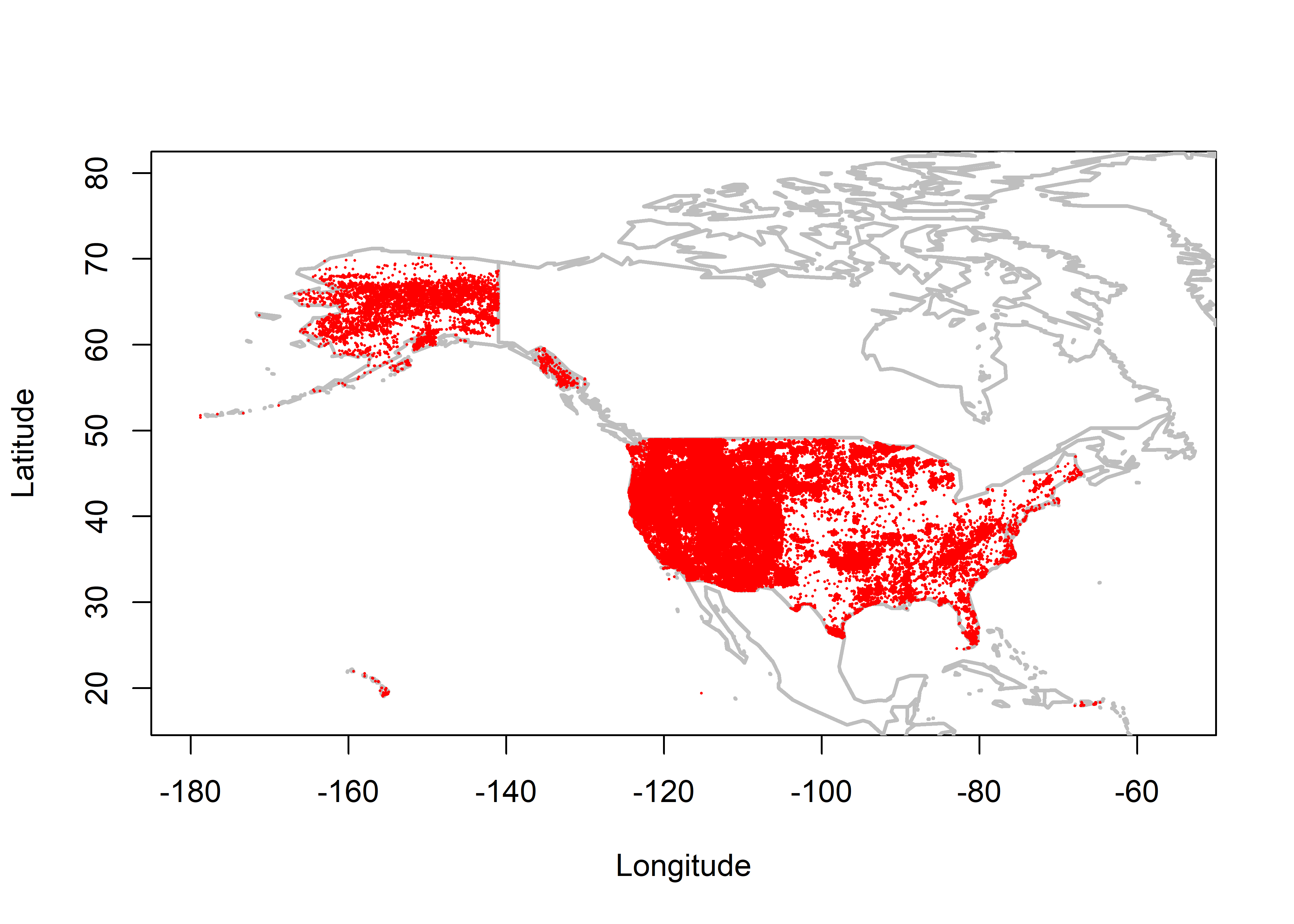
1.3.2 Time series
Number of fires by different (general) causes, and by agency and cause
table(fwfod$CAUSE)##
## Human Natural Undetermined Unknown
## 326975 256607 87 90table(fwfod$ORGANIZATI,fwfod$CAUSE)##
## Human Natural Undetermined Unknown
## BIA 90629 19090 0 25
## BLM 44721 61386 0 37
## BOR 3 8 0 0
## FS 155437 160143 0 0
## FWS 21397 6224 87 0
## NPS 14788 9756 0 28Get the startday number (startdaynum day number in the year), and month (startmon) and day (startday) of each record.
library(lubridate)
fwfod$STARTDATED <- as.character(fwfod$STARTDATED)
fwfod$STARTDATED <- as.Date(fwfod$STARTDATED)
fwfod$startdaynum <- yday((strptime(fwfod$STARTDATED, "%Y-%m-%d")))
fwfod$startday <- as.numeric(format(fwfod$STARTDATED, format="%d"))
fwfod$startmon <- as.numeric(format(fwfod$STARTDATED, format="%m"))
fwfod$startyear <- as.numeric(format(fwfod$STARTDATED, format="%Y"))
Convert acres to hectares
fwfod$AREA <- fwfod$TOTALACRES * 0.404686Check startyear values
## check records
table(fwfod$startyear)
##
## 213 1013 1980 1981 1982 1983 1984 1985 1986 1987 1988 1989 1990 1991 1992 1993 1994
## 1 1 8954 10328 6278 6451 9147 10390 15489 19422 19908 17797 17830 17332 19320 14300 23666
## 1995 1996 1997 1998 1999 2000 2001 2002 2003 2004 2005 2006 2007 2008 2009 2010 2011
## 16754 20189 14309 18183 21657 23064 21303 20639 22155 19210 19508 24576 20414 15651 15742 14946 15801
## 2012 2013 2014
## 16320 16378 15475Two records have startyear values less than 1980. Find them:
fwfod[fwfod$startyear == 213,]## OBJECTID ORGANIZATI UNIT SUBUNIT SUBUNIT2 FIREID FIRENAME FIRENUMBER FIRECODE CAUSE SPECCAUSE
## 624553 6741 FS 6 617 <NA> 1519270 BENTON 98 P6RK2Q Natural 1
## STATCAUSE SIZECLASS SIZECLASSN PROTECTION FIREPROTTY FIRETYPE YEAR_ STARTDATED CONTRDATED
## 624553 1 B 2 0 0 0 2013 0213-08-11 2013-08-12
## OUTDATED GACC DISPATCH GACCN STATE STATE_FIPS FIPS
## 624553 2013-08-17 NWCC Central Washington Interagency Comm Center 106 Washington 53 53
## DLATITUDE DLONGITUDE TOTALACRES TRPGENCAUS TRPSPECCAU validpt startdaynum startday startmon
## 624553 46.705 -120.9381 2.2 0 0 1 223 11 8
## startyear AREA
## 624553 213 0.8903092fwfod[fwfod$startyear == 1013,]## OBJECTID ORGANIZATI UNIT SUBUNIT SUBUNIT2 FIREID FIRENAME FIRENUMBER FIRECODE CAUSE SPECCAUSE
## 619816 2004 FS 3 302 <NA> 1514755 CHACON 71 P3EKV1 Natural 1
## STATCAUSE SIZECLASS SIZECLASSN PROTECTION FIREPROTTY FIRETYPE YEAR_ STARTDATED CONTRDATED
## 619816 1 A 1 0 0 0 2013 1013-07-26 2013-08-05
## OUTDATED GACC DISPATCH GACCN STATE STATE_FIPS FIPS DLATITUDE DLONGITUDE TOTALACRES
## 619816 2013-08-05 SWCC Taos Zone 110 New Mexico 35 35 36.54722 -106.305 0.25
## TRPGENCAUS TRPSPECCAU validpt startdaynum startday startmon startyear AREA
## 619816 0 0 1 207 26 7 1013 0.1011715Fix the two records
fwfod[fwfod$startyear == 213,]$STARTDATED <- "2013-08-11"
fwfod[fwfod$startyear == 213,]$startyear <- 2013
fwfod[fwfod$startyear == 1013,]$STARTDATED <- "2013-07-26"
fwfod[fwfod$startyear == 1013,]$startyear <- 2013
table(fwfod$startyear)
##
## 1980 1981 1982 1983 1984 1985 1986 1987 1988 1989 1990 1991 1992 1993 1994 1995 1996
## 8954 10328 6278 6451 9147 10390 15489 19422 19908 17797 17830 17332 19320 14300 23666 16754 20189
## 1997 1998 1999 2000 2001 2002 2003 2004 2005 2006 2007 2008 2009 2010 2011 2012 2013
## 14309 18183 21657 23064 21303 20639 22155 19210 19508 24576 20414 15651 15742 14946 15801 16320 16380
## 2014
## 15475Number of fires per year
hist(fwfod$startyear, xlim=c(1980,2015), ylim=c(0,40000),breaks=seq(1979.5,2014.5,by=1))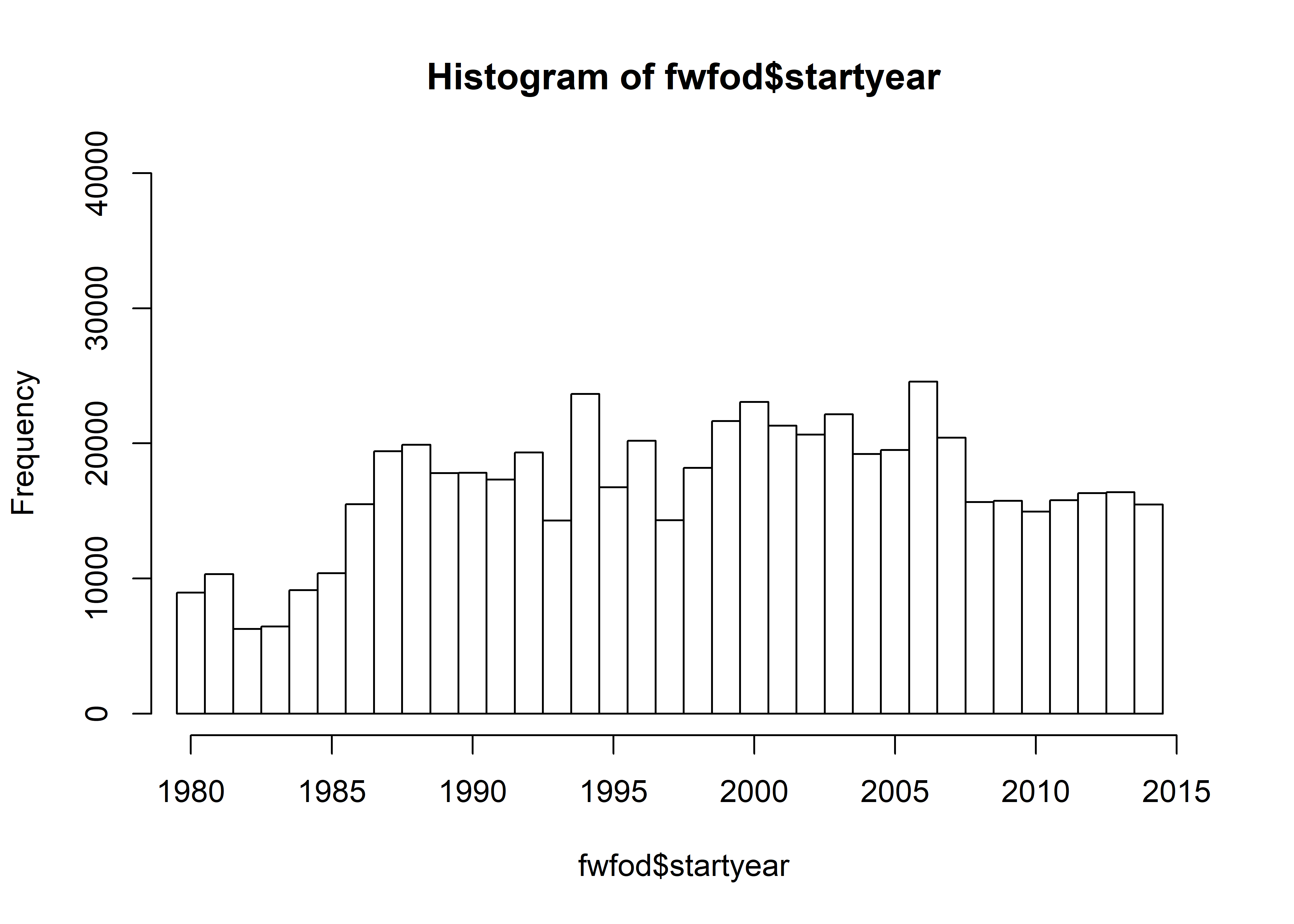
table(fwfod$startyear)##
## 1980 1981 1982 1983 1984 1985 1986 1987 1988 1989 1990 1991 1992 1993 1994 1995 1996
## 8954 10328 6278 6451 9147 10390 15489 19422 19908 17797 17830 17332 19320 14300 23666 16754 20189
## 1997 1998 1999 2000 2001 2002 2003 2004 2005 2006 2007 2008 2009 2010 2011 2012 2013
## 14309 18183 21657 23064 21303 20639 22155 19210 19508 24576 20414 15651 15742 14946 15801 16320 16380
## 2014
## 15475hist(fwfod$startyear[fwfod$CAUSE == "Natural"], xlim=c(1980,2015), ylim=c(0,40000),
breaks=seq(1979.5,2014.5,by=1), main="fwfod Natural")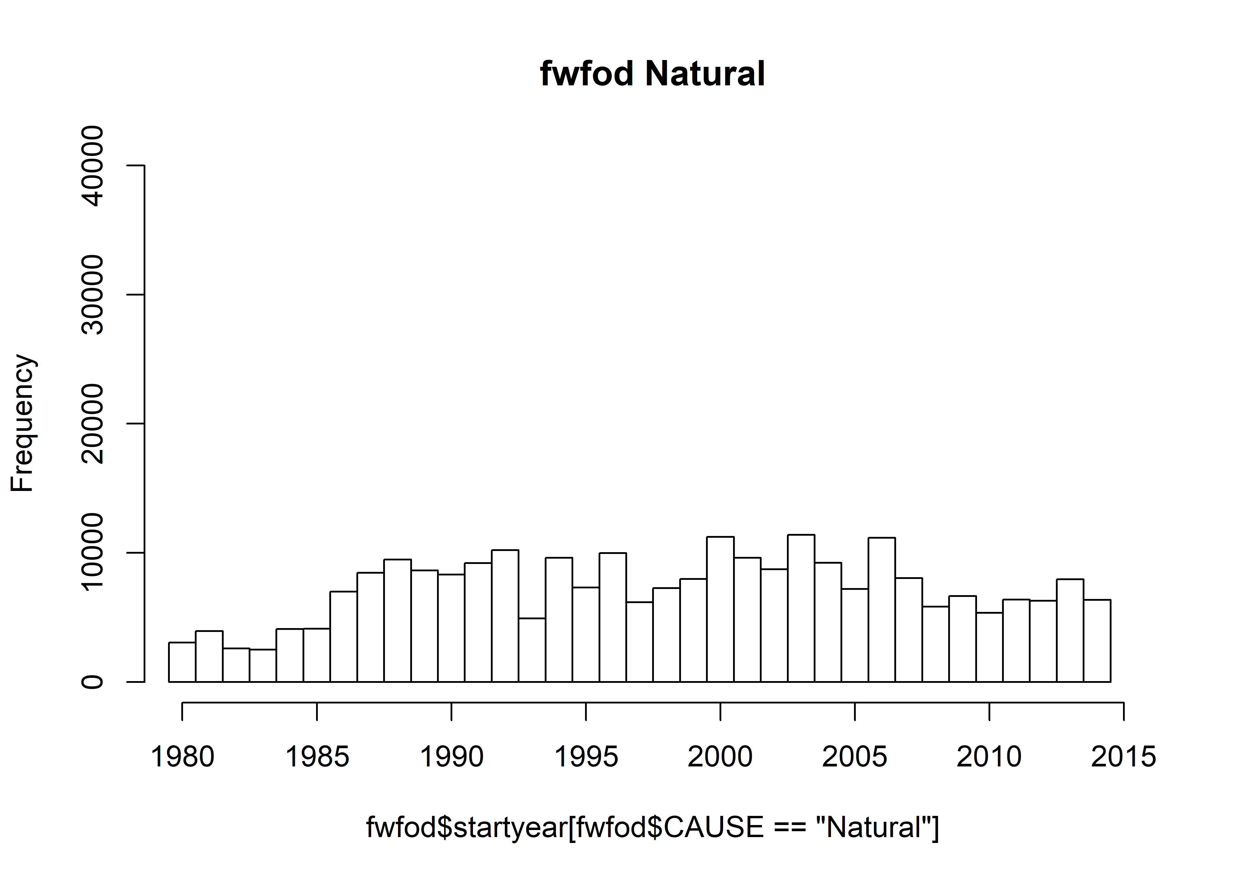
table(fwfod$startyear[fwfod$CAUSE == "Natural"])##
## 1980 1981 1982 1983 1984 1985 1986 1987 1988 1989 1990 1991 1992 1993 1994 1995 1996
## 3069 3959 2598 2517 4115 4127 7003 8470 9490 8653 8332 9200 10207 4925 9624 7321 9989
## 1997 1998 1999 2000 2001 2002 2003 2004 2005 2006 2007 2008 2009 2010 2011 2012 2013
## 6185 7280 7985 11248 9632 8739 11392 9243 7209 11162 8055 5840 6656 5358 6391 6305 7961
## 2014
## 6367hist(fwfod$startyear[fwfod$CAUSE == "Human"], xlim=c(1980,2015), ylim=c(0,40000),
breaks=seq(1979.5,2014.5,by=1), main="fwfod Human")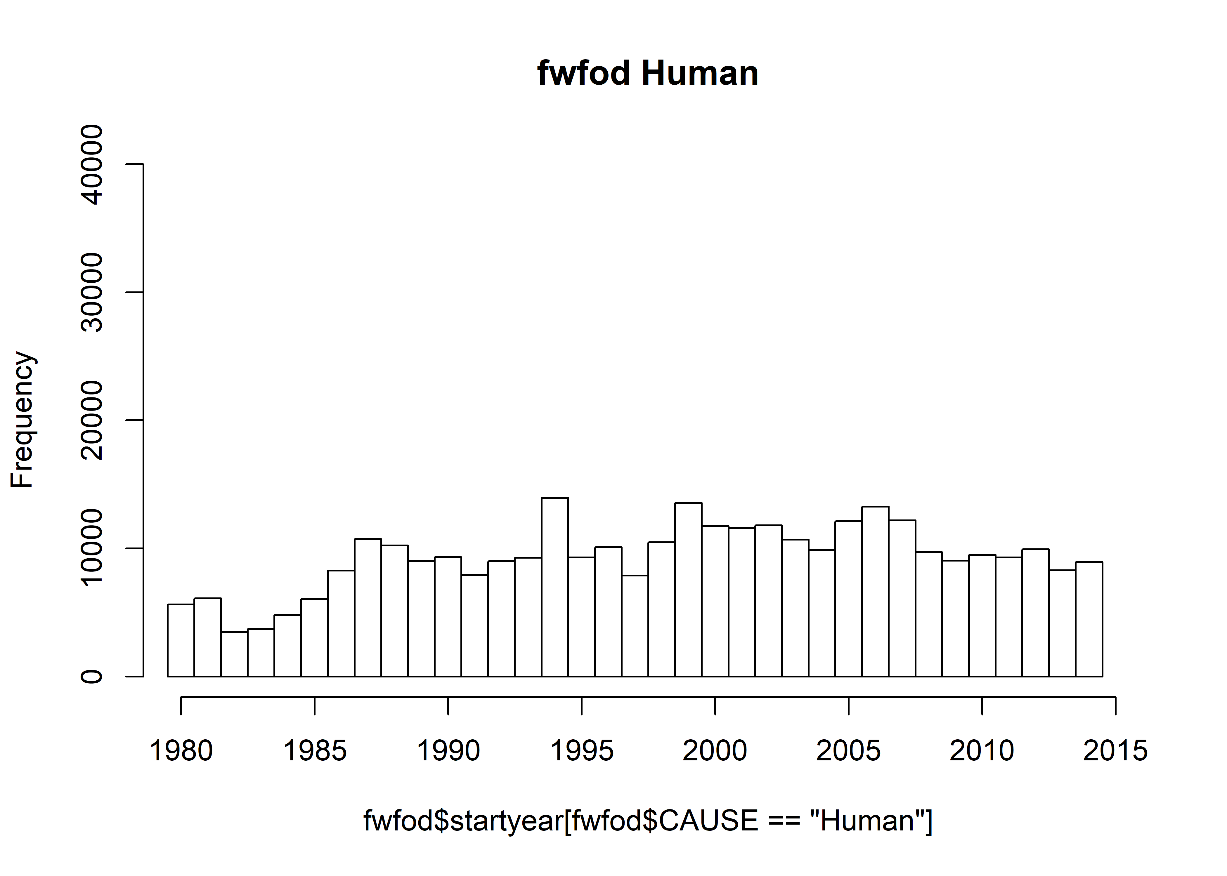
table(fwfod$startyear[fwfod$CAUSE == "Human"])##
## 1980 1981 1982 1983 1984 1985 1986 1987 1988 1989 1990 1991 1992 1993 1994 1995 1996
## 5641 6118 3467 3720 4806 6062 8272 10743 10231 9034 9333 7933 9006 9280 13962 9299 10101
## 1997 1998 1999 2000 2001 2002 2003 2004 2005 2006 2007 2008 2009 2010 2011 2012 2013
## 7886 10489 13574 11733 11593 11810 10690 9886 12130 13269 12195 9705 9041 9499 9307 9935 8294
## 2014
## 8931Get the total area burned by year
total_by_year <- tapply(fwfod$AREA, fwfod$YEAR_, sum)
total_by_year
## 1980 1981 1982 1983 1984 1985 1986 1987 1988 1989
## 376937.7 772901.1 174664.0 272892.2 496682.0 888544.9 619901.7 951178.4 3771214.7 610271.2
## 1990 1991 1992 1993 1994 1995 1996 1997 1998 1999
## 1610359.9 1142398.2 606096.8 759900.1 1323328.4 483741.4 1966609.8 1077143.9 437718.8 1983707.5
## 2000 2001 2002 2003 2004 2005 2006 2007 2008 2009
## 3290616.5 897304.4 3768737.2 1891143.8 3970058.5 5129648.1 2997866.5 3150657.8 1353575.6 2421749.2
## 2010 2011 2012 2013 2014
## 1213475.7 1882140.1 2818697.7 1762547.0 1368782.9year <- as.numeric(unlist(dimnames(total_by_year)))
total_by_year <- as.numeric(total_by_year)
plot(total_by_year ~ year, pch=16, type="o", lwd=3, col="red", main="Total Area Burned (ha) (U.S. All)")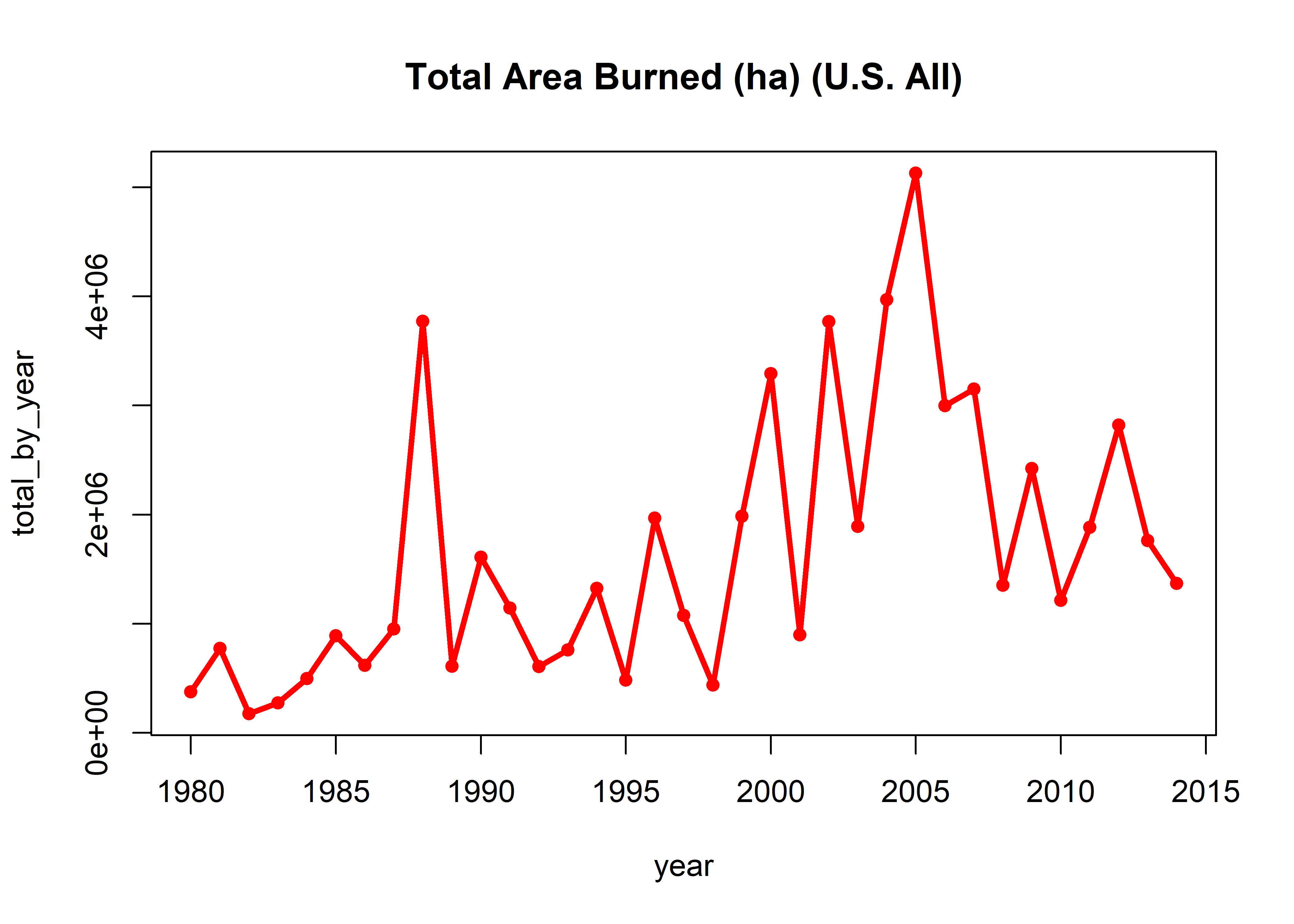
Mean area burned by year.
mean_by_year <- tapply(fwfod$AREA, fwfod$YEAR_, mean)
mean_by_year
## 1980 1981 1982 1983 1984 1985 1986 1987 1988 1989
## 42.09713 74.83550 27.82160 42.30230 54.29999 85.51924 40.02206 48.97428 189.43212 34.29068
## 1990 1991 1992 1993 1994 1995 1996 1997 1998 1999
## 90.31744 65.91266 31.37147 53.13987 55.91686 28.87319 97.40997 75.27737 24.07297 91.59660
## 2000 2001 2002 2003 2004 2005 2006 2007 2008 2009
## 142.67328 42.12103 182.60270 85.35968 206.66624 262.95100 121.98350 154.33809 86.48493 153.83999
## 2010 2011 2012 2013 2014
## 81.19067 119.13033 172.93685 107.54451 88.37129year <- as.numeric(unlist(dimnames(mean_by_year)))
mean_by_year <- as.numeric(mean_by_year)
plot(mean_by_year ~ year, pch=16, type="o", lwd=3, col="red", main="Mean Area Burned (ha) (U.S. All)")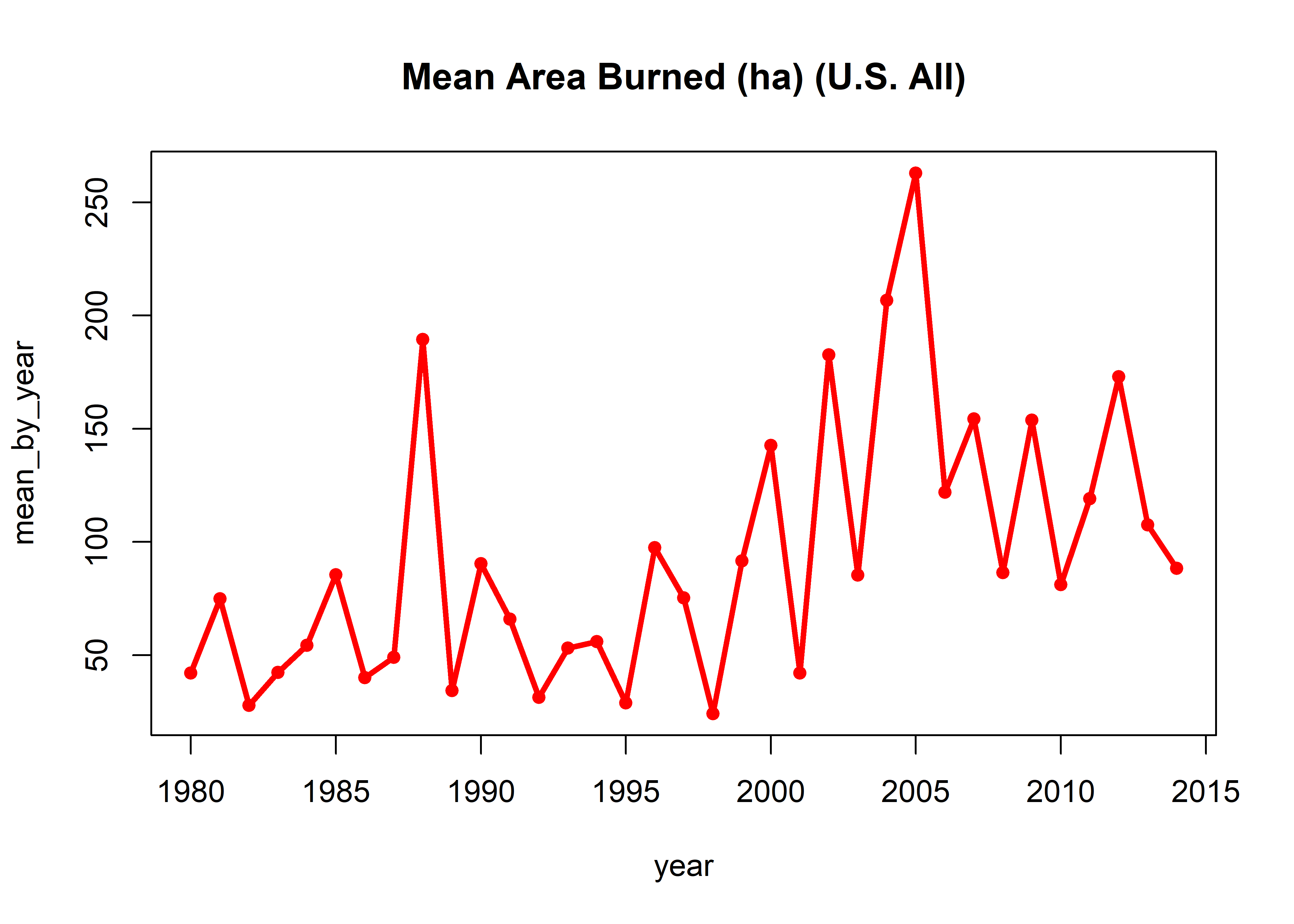
2 Start-day problem
The start-day problem is described more elaborately in the file fwfod_startday_features_04.html.
2.1 Histograms
Histograms of start-day number (startdaynum) for all data, human and lightning:
hist(fwfod$startdaynum, breaks=seq(-0.5,366.5,by=1), freq=-TRUE, ylim=c(0,6000), xlim=c(0,400))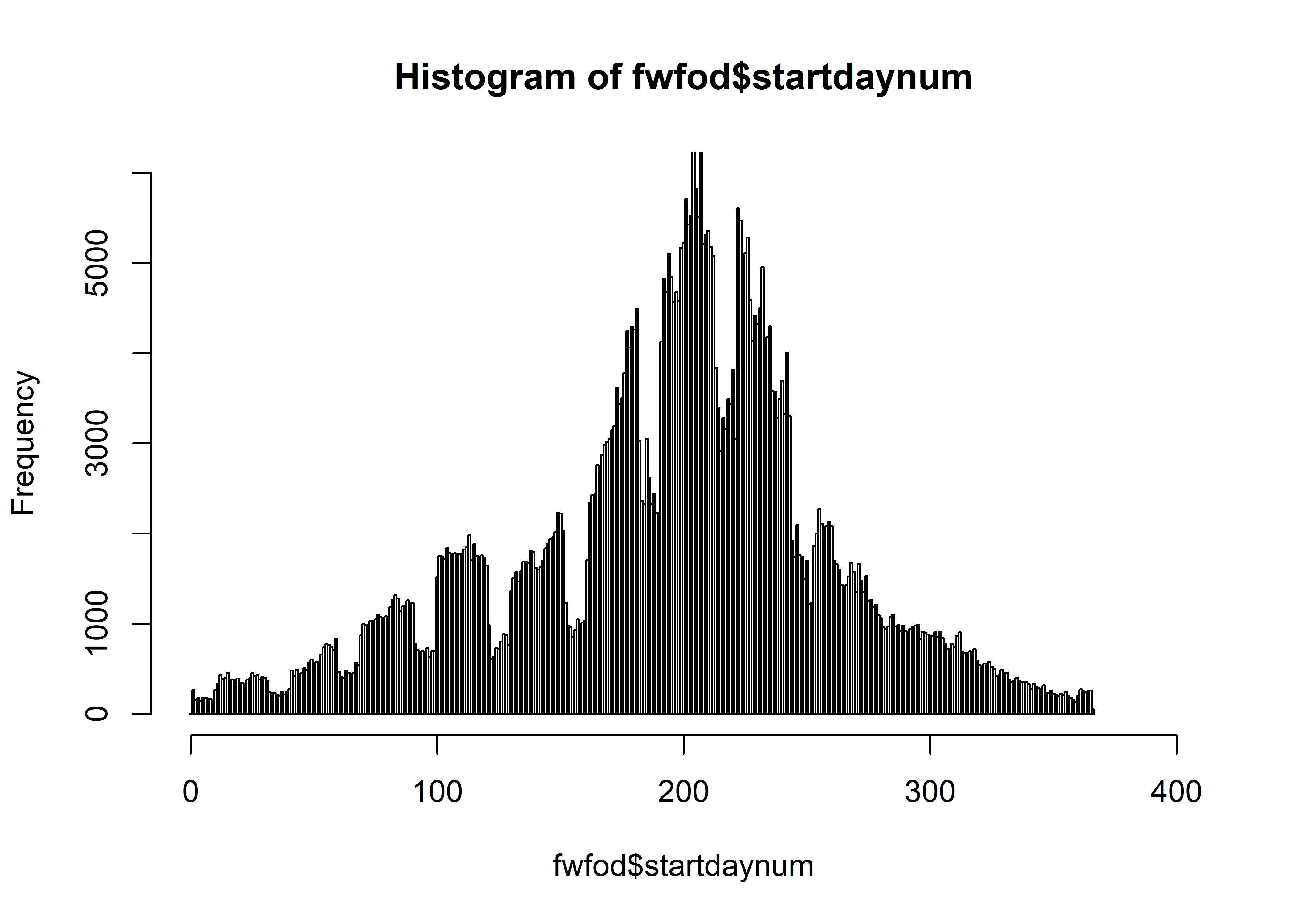
hist(fwfod$startdaynum[fwfod$CAUSE=="Human"], breaks=seq(-0.5,366.5,by=1), freq=-TRUE,
  xlim=c(0,400), ylim=c(0,6000))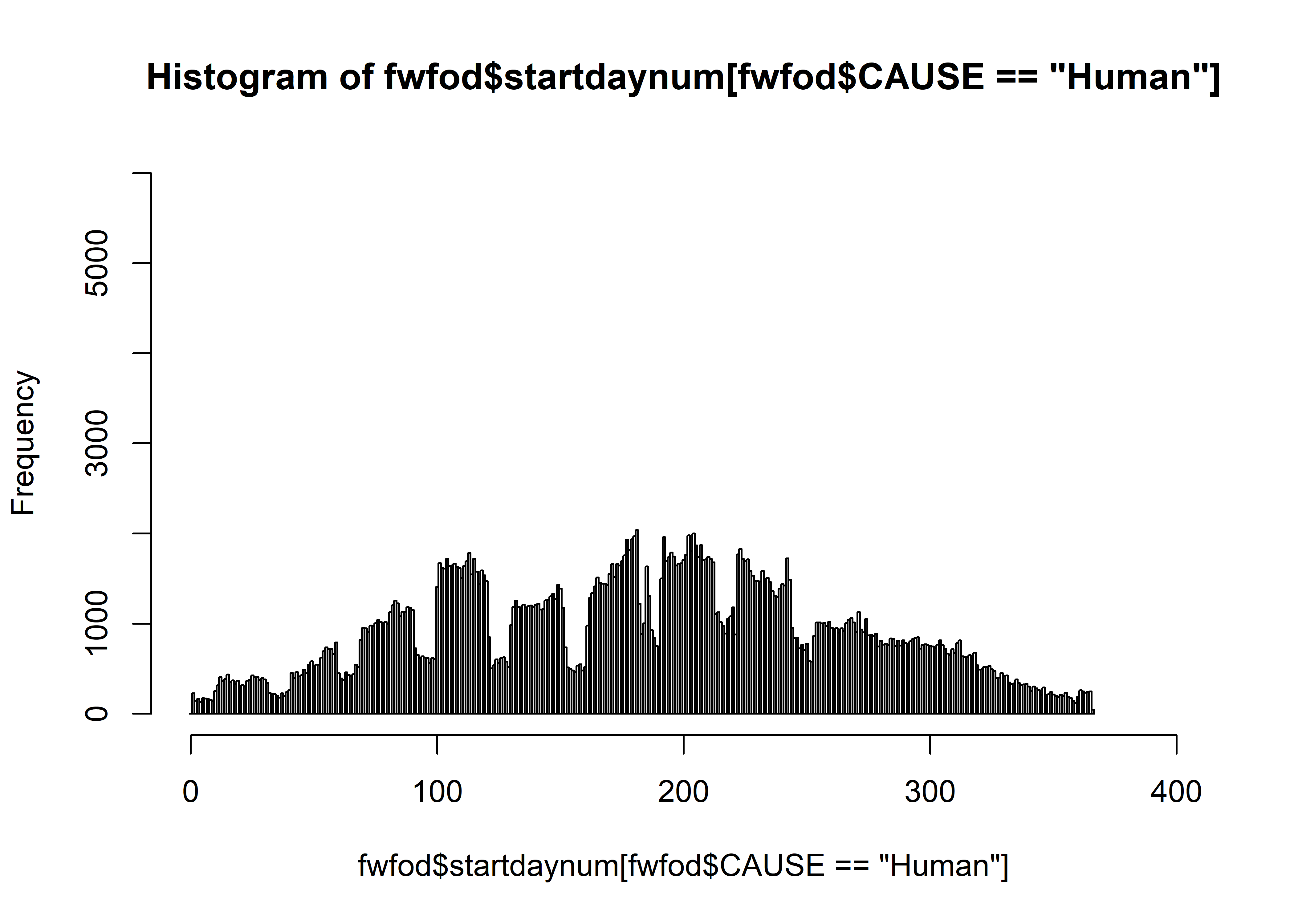
hist(fwfod$startdaynum[fwfod$CAUSE=="Natural"], breaks=seq(-0.5,366.5,by=1), freq=-TRUE,
  xlim=c(0,400), ylim=c(0,6000))
Note the obvious “chunks” in the histograms, corresponding to days 1-9 in each month (except Oct-Dec).
Histograms of the start day within each month over all months. Each day number should be roughly equally likely, but days 1 through 9 occur less frequently:
oldpar <- par(mfrow=c(1,3))
hist(fwfod$startday, breaks=seq(-0.5,31.5,by=1), freq=-TRUE, ylim=c(0,60000))
hist(fwfod$startday[fwfod$CAUSE=="Natural"], breaks=seq(-0.5,31.5,by=1), freq=-TRUE, ylim=c(0,30000))
hist(fwfod$startday[fwfod$CAUSE=="Human"], breaks=seq(-0.5,31.5,by=1), freq=-TRUE, ylim=c(0,30000))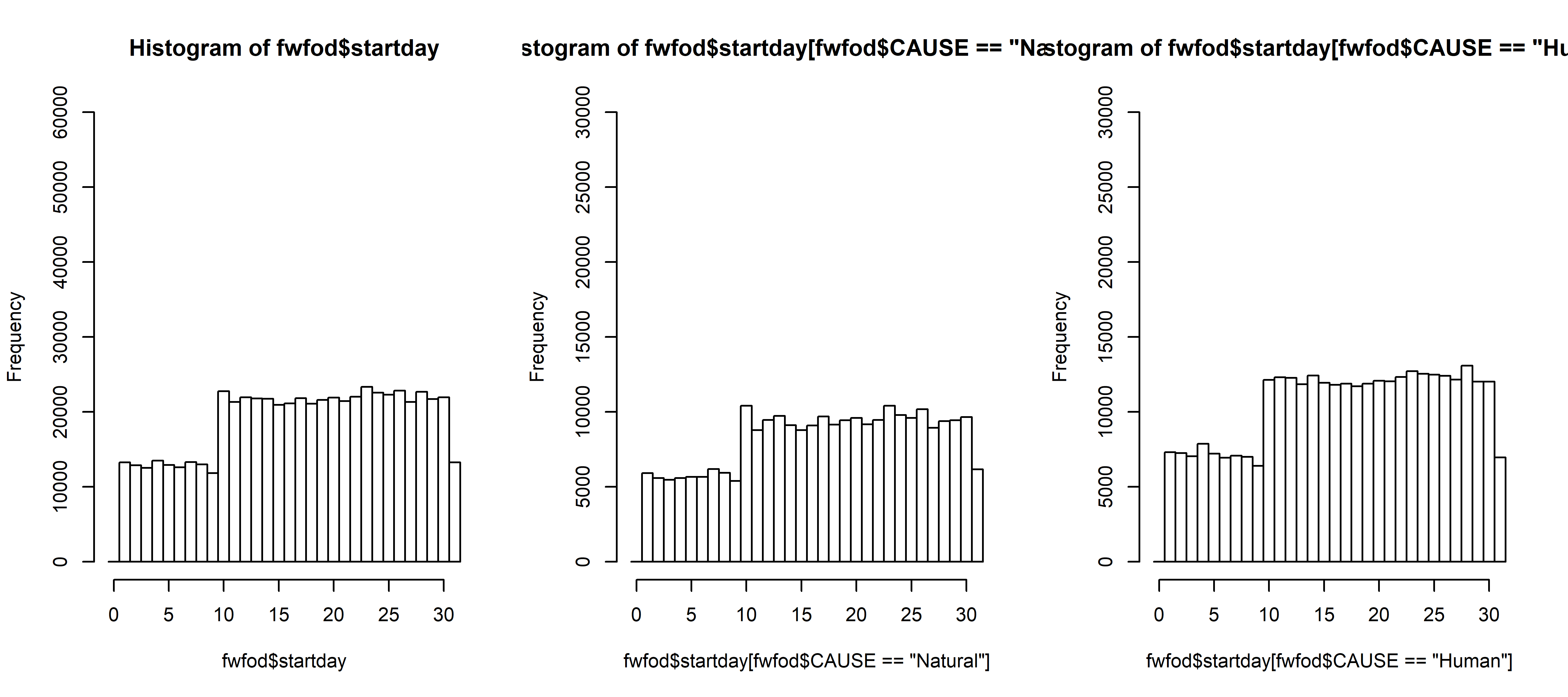
par(oldpar)By agency:
oldpar <- par(mfrow=c(1,3))
hist(fwfod$startday[fwfod$ORGANIZATI =="BIA"], breaks=seq(-0.5,31.5,by=1), freq=-TRUE, ylim=c(0,10000))
hist(fwfod$startday[fwfod$ORGANIZATI=="BLM"], breaks=seq(-0.5,31.5,by=1), freq=-TRUE, ylim=c(0,10000))
hist(fwfod$startday[fwfod$ORGANIZATI=="BOR"], breaks=seq(-0.5,31.5,by=1), freq=-TRUE, ylim=c(0,10))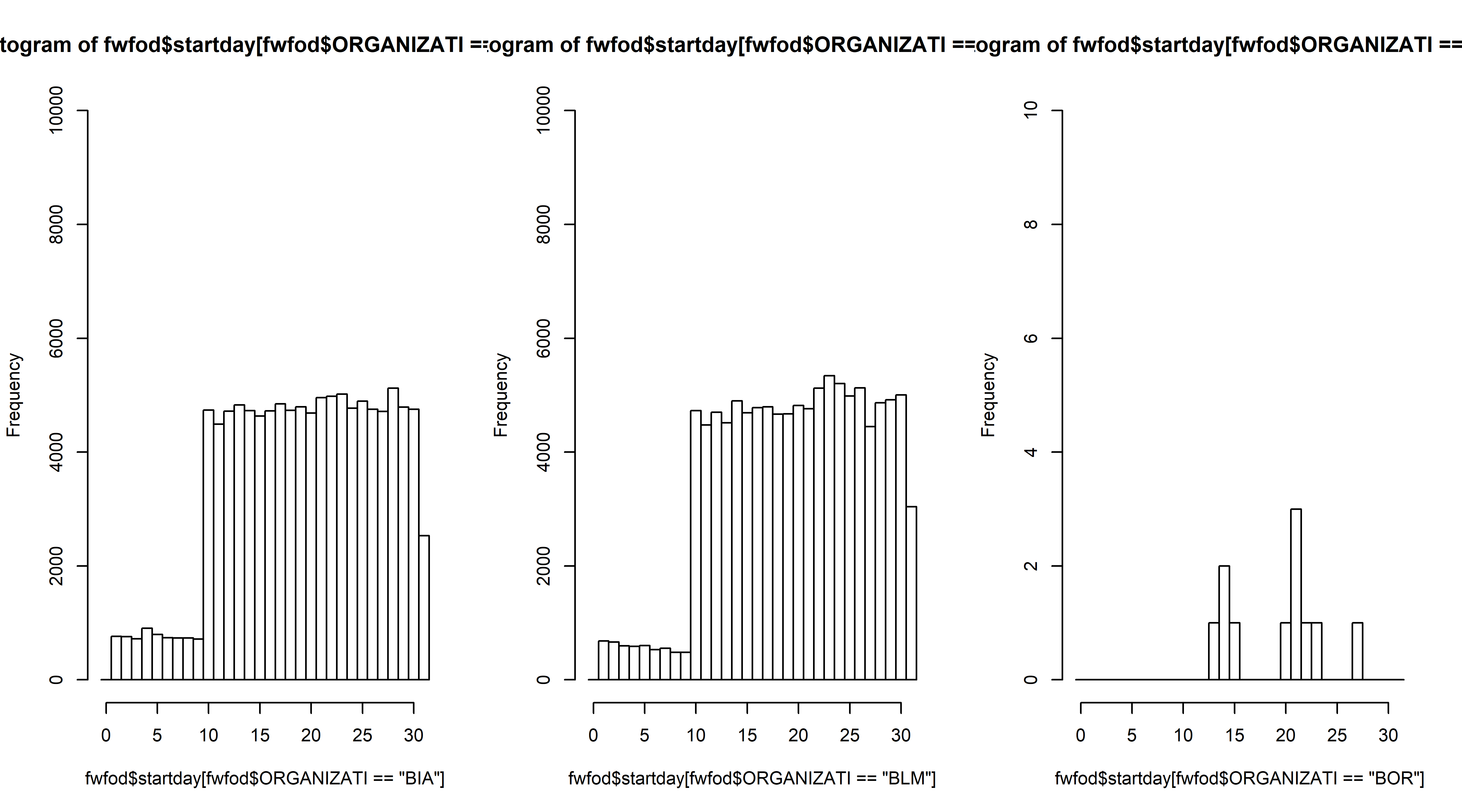
par(oldpar)oldpar <- par(mfrow=c(1,3))
hist(fwfod$startday[fwfod$ORGANIZATI=="FS"], breaks=seq(-0.5,31.5,by=1), freq=-TRUE, ylim=c(0,20000))
hist(fwfod$startday[fwfod$ORGANIZATI=="FWS"], breaks=seq(-0.5,31.5,by=1), freq=-TRUE, ylim=c(0,10000))
hist(fwfod$startday[fwfod$ORGANIZATI=="NPS"], breaks=seq(-0.5,31.5,by=1), freq=-TRUE, ylim=c(0,10000))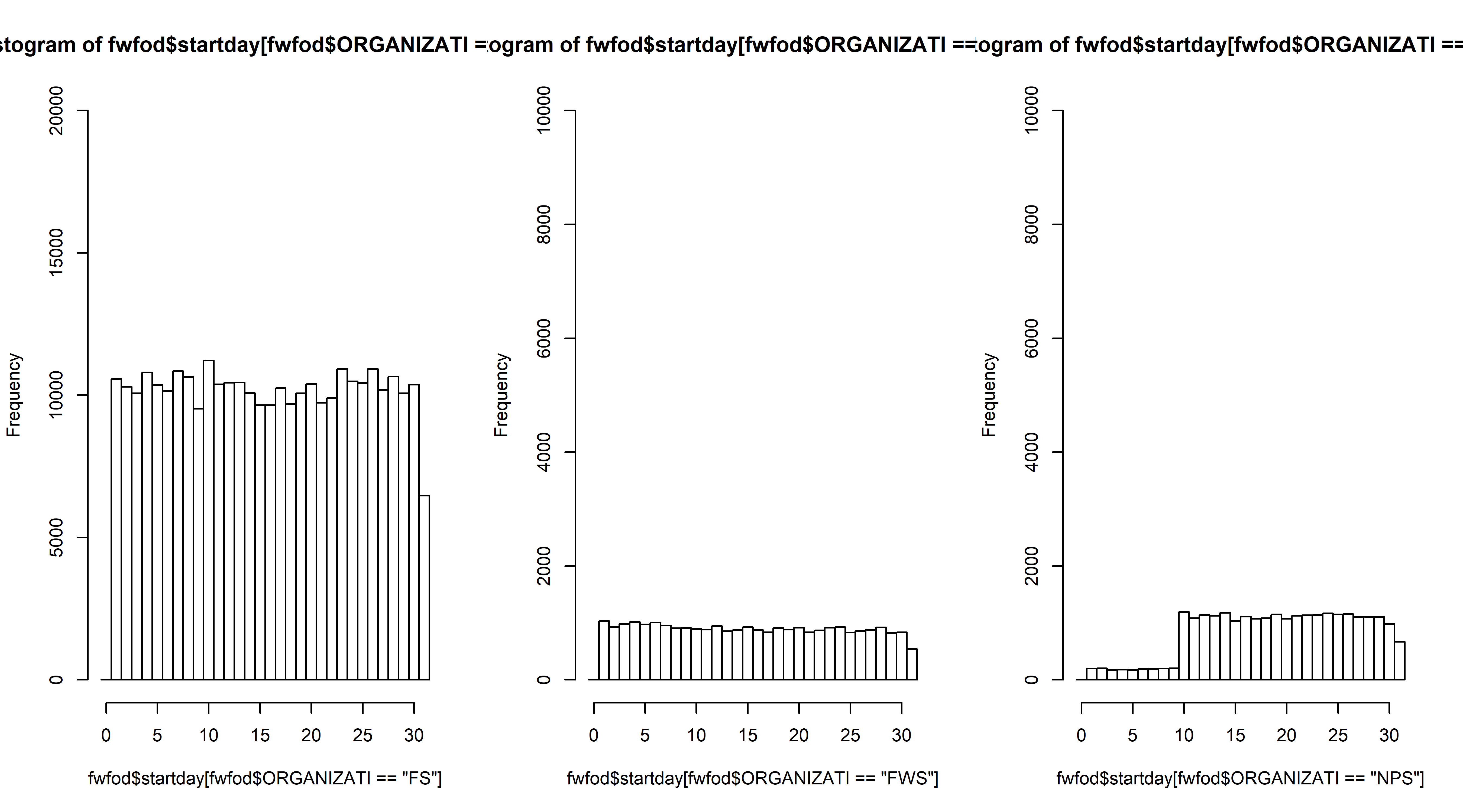
par(oldpar)Agencies with names that begin with an “F” do not seem to be affected.
Examine start-day frequecny by size of fire:
sizecut <- 100.0
fwfod.big <- fwfod[fwfod$TOTALACRES > sizecut,]
table(fwfod.big$CAUSE)
##
## Human Natural Undetermined Unknown
## 15360 13647 14 7hist(fwfod.big$startday, breaks=seq(-0.5,31.5,by=1), freq=-TRUE)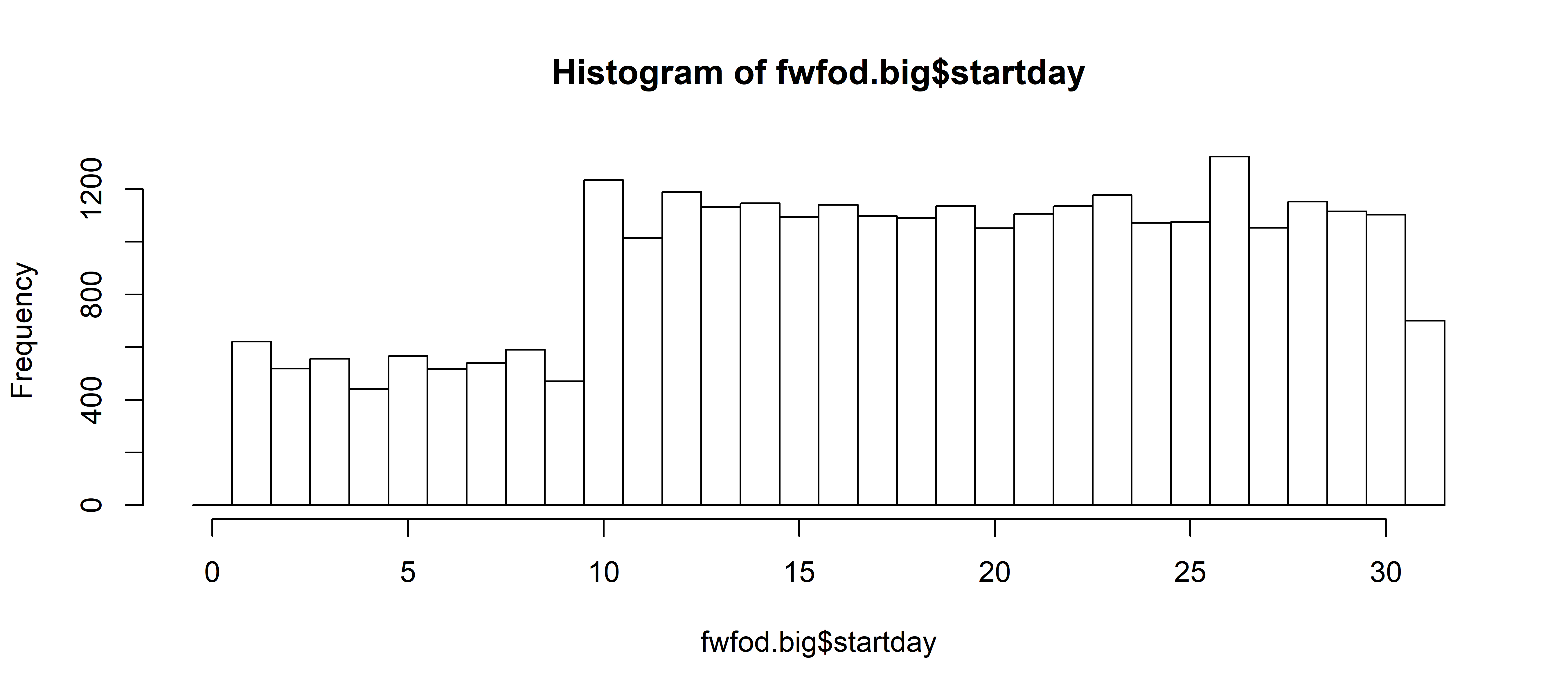
hist(fwfod.big$startday[fwfod$CAUSE=="Natural"], breaks=seq(-0.5,31.5,by=1), freq=-TRUE)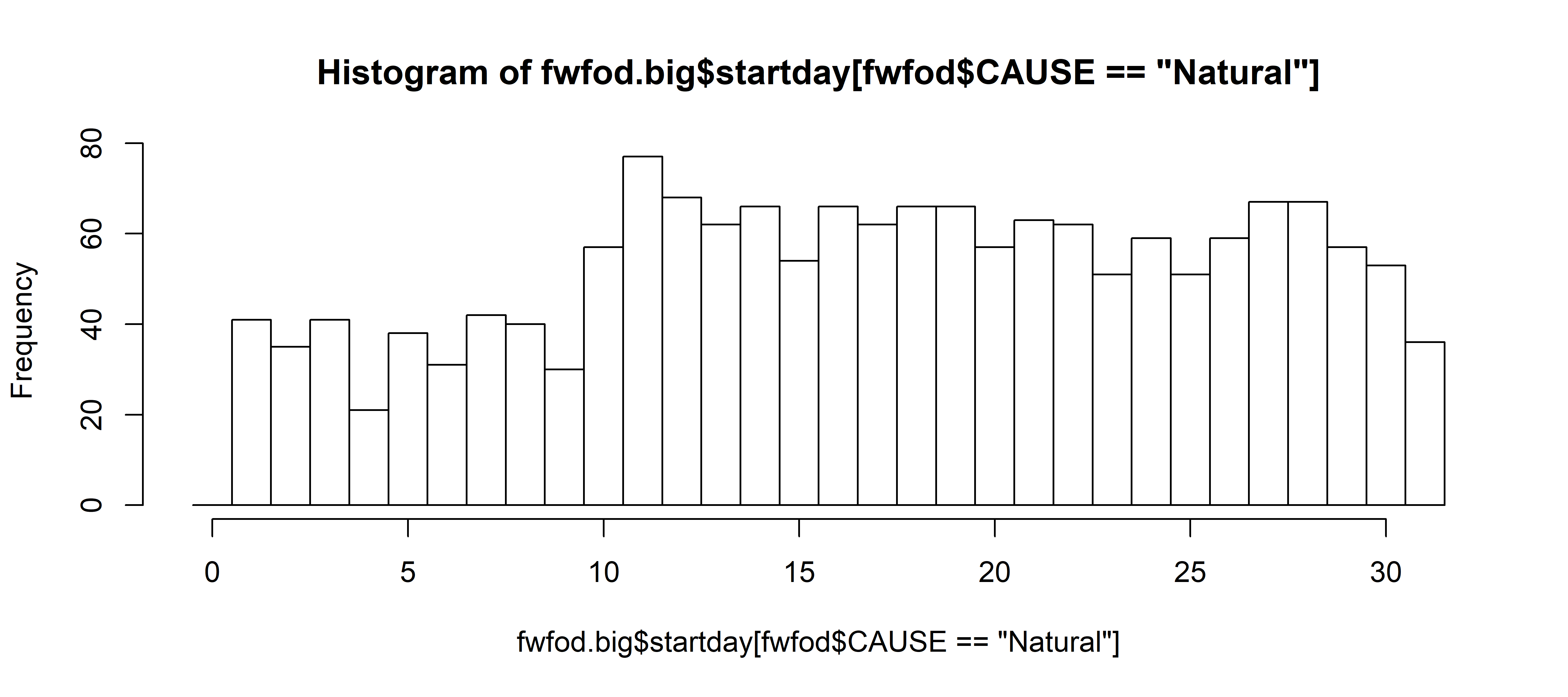
hist(fwfod.big$startday[fwfod$CAUSE=="Human"], breaks=seq(-0.5,31.5,by=1), freq=-TRUE)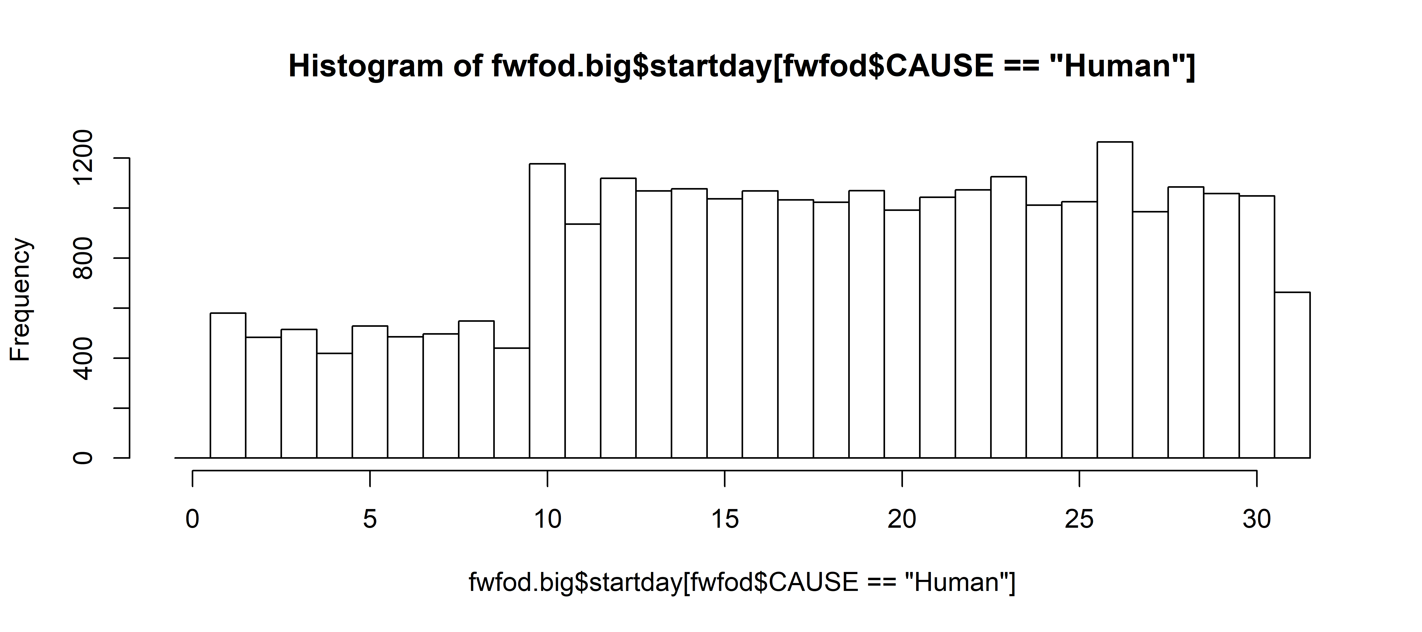
2.2 Mosaic plots
Plots of relative numbers of fires days 1-9 and 10-31
fwfod$startday2 <- fwfod$startday
fwfod$startday2 <- ifelse(fwfod$startday2 <= 9,  fwfod$startday2 <- "1-9", fwfod$startday2 <- "10-31")
table(fwfod$startday2)
##
## 1-9 10-31
## 115690 473198fwfod.table <- table(fwfod$YEAR_, fwfod$startday2)
fwfod.year <- as.integer(row.names(fwfod.table))
fwfod.ratio <- fwfod.table[,1]/fwfod.table[,2]
mosaicplot(fwfod.table, color=c(3,4), cex.axis=0.6, las=3, main="Start Day in Month by Year")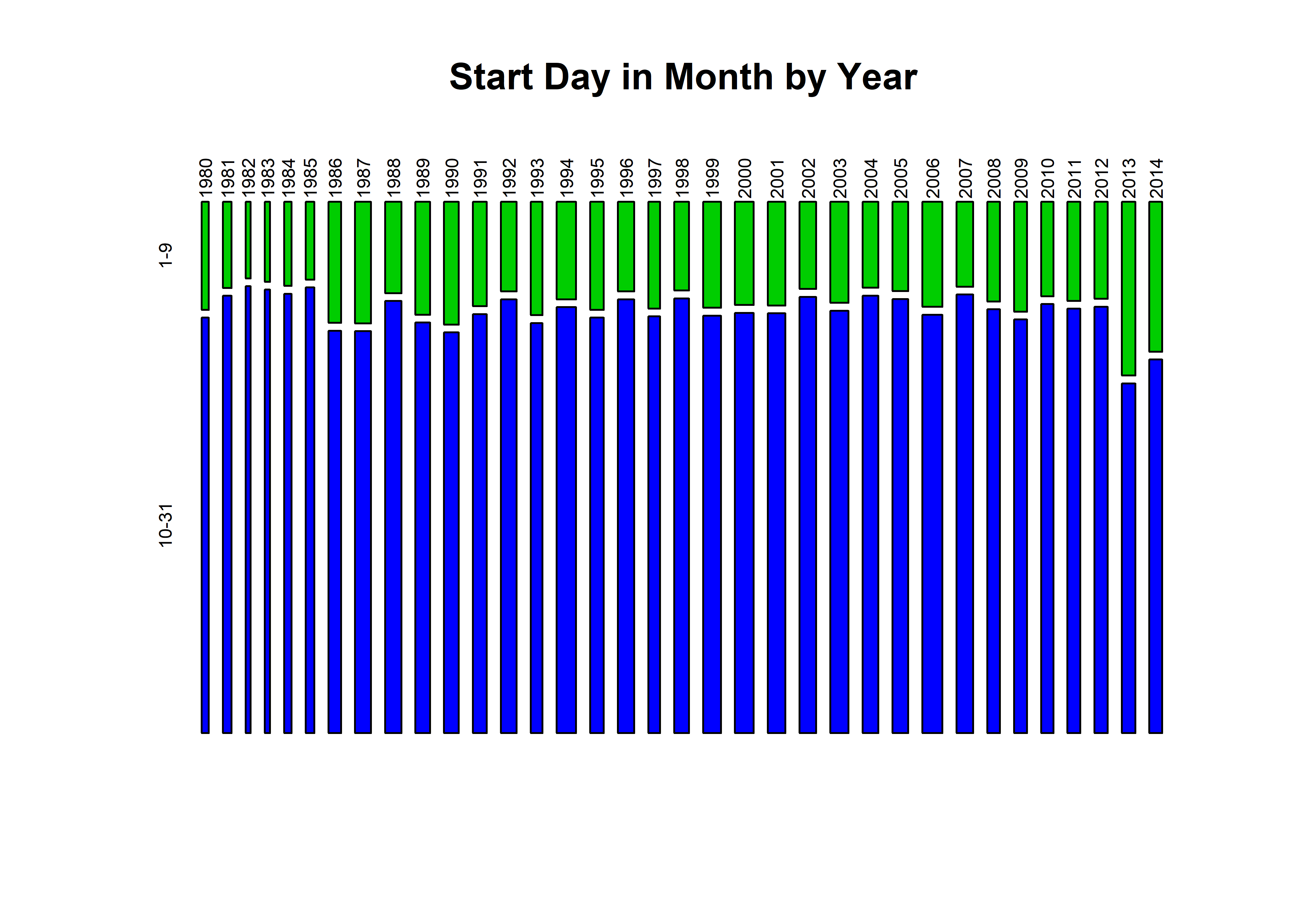
plot(fwfod.year, fwfod.ratio, pch=16, type="o", lwd=3, col="red")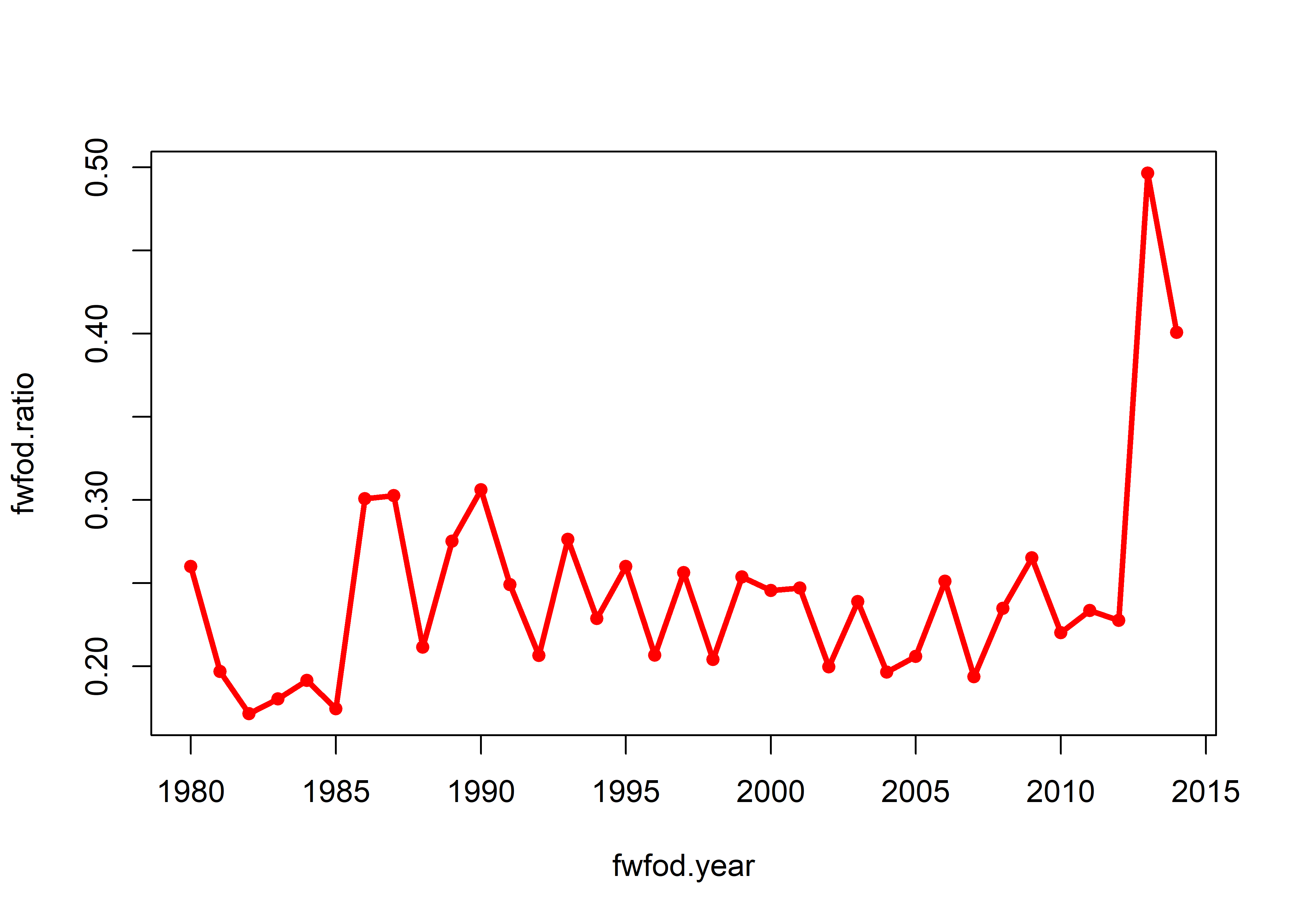
The mosaic plot shows that throughout the record, the number of fires in days 1-9, are underrepresented. The expected number of fires in days 1-9 is 0.296 = 9/30.4, where 30.4 = 365.25/12, while the observed proportion is 0.244 = 115690/473198.
The mosaic plots also show that there is a discontinuity in the annual number of fires between 1985 and 1986, and possibly also between 2007 and 2008. Only in 2013 and 2014 do the proportions of fires in the the first third and last two-thirds of the months seem reasonable.
Examine the relative proportions of first-third vs. last-two-thirds start days by individual months:
fwfod.table.start <- table(fwfod$startmon, fwfod$startday2)
mosaicplot(fwfod.table.start, color=c(3,4), cex.axis=0.6, las=3, main="Start Day in Month by Month")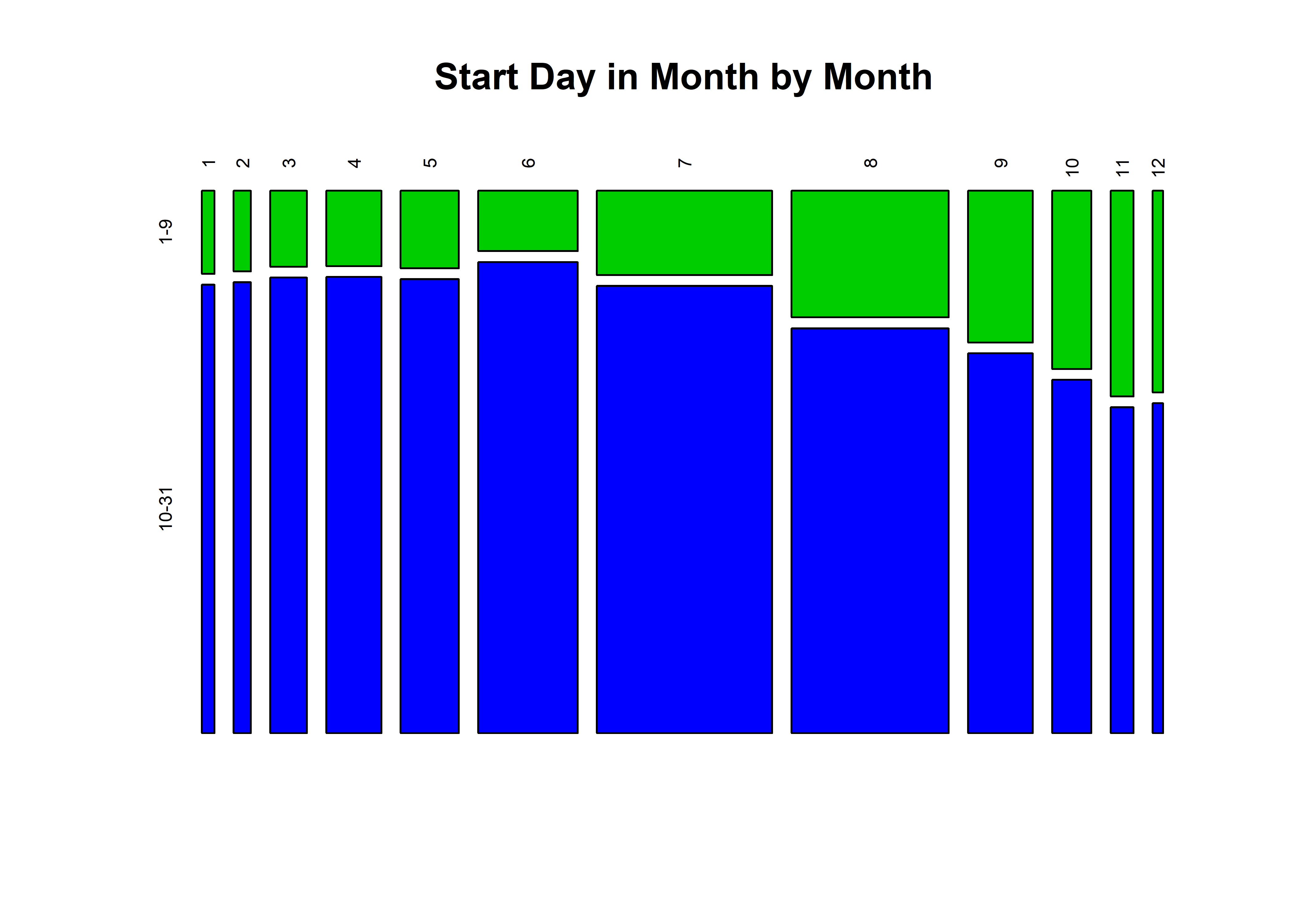
It seems likely that there was a month/day-in-month transposition at some point, where the problem seems to be worse for months 1 through 0 (January through September).
More mosaic plots, showing the distribution of fires by month and year.
fwfod.tablemon <- table(fwfod$YEAR_, fwfod$startmon)
mosaicplot(fwfod.tablemon, color=monthcolors, cex.axis=0.6, las=3, main="All Fires")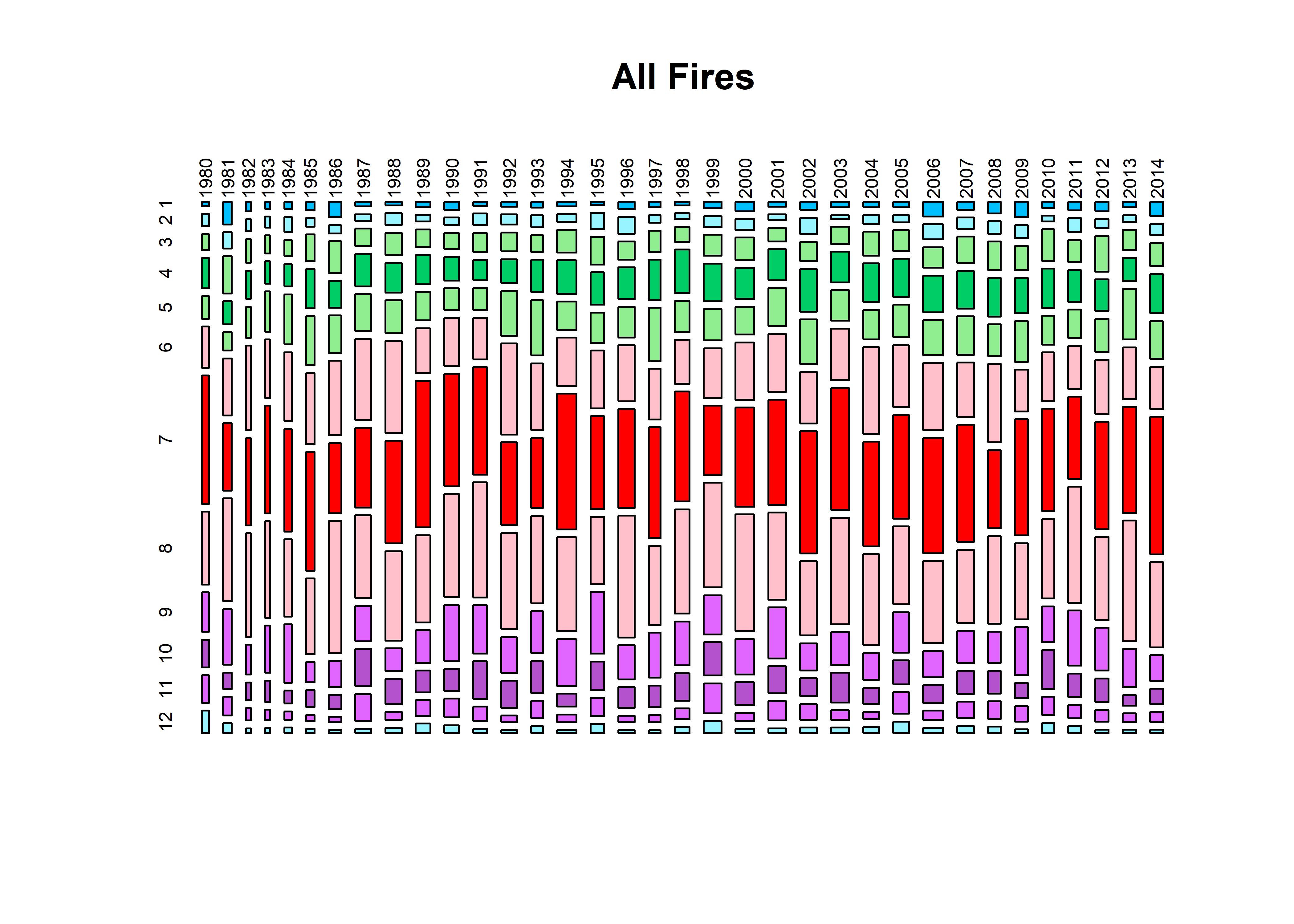
fwfod.tablemon.n <- table(fwfod$YEAR_[fwfod$CAUSE=="Natural"], fwfod$startmon[fwfod$CAUSE=="Natural"])
mosaicplot(fwfod.tablemon.n, color=monthcolors, cex.axis=0.6, las=3, main="Natural Fires")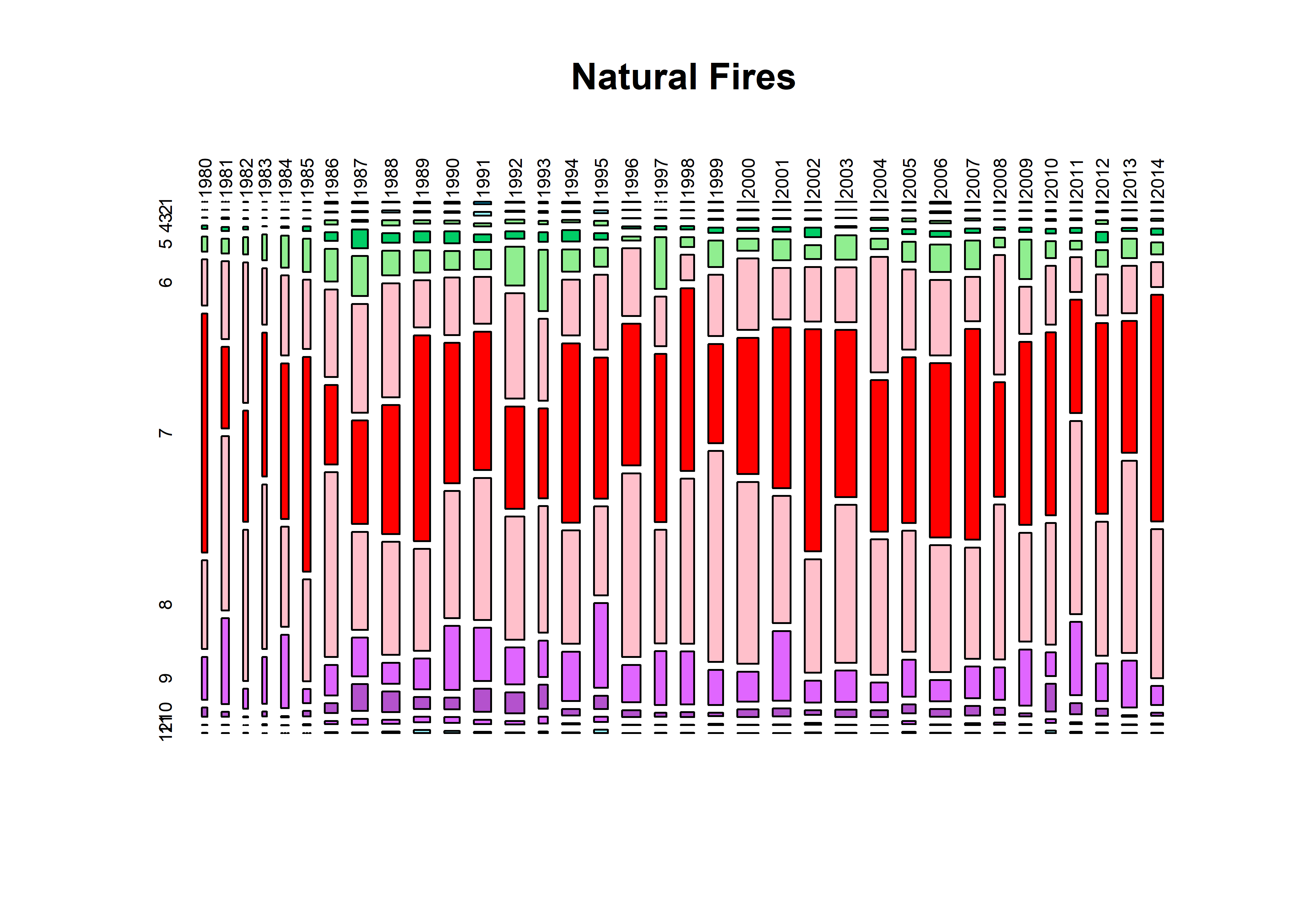
fwfod.tablemon.h <- table(fwfod$YEAR_[fwfod$CAUSE=="Human"], fwfod$startmon[fwfod$CAUSE=="Human"])
mosaicplot(fwfod.tablemon.h, color=monthcolors, cex.axis=0.6, las=3, main="Human Fires")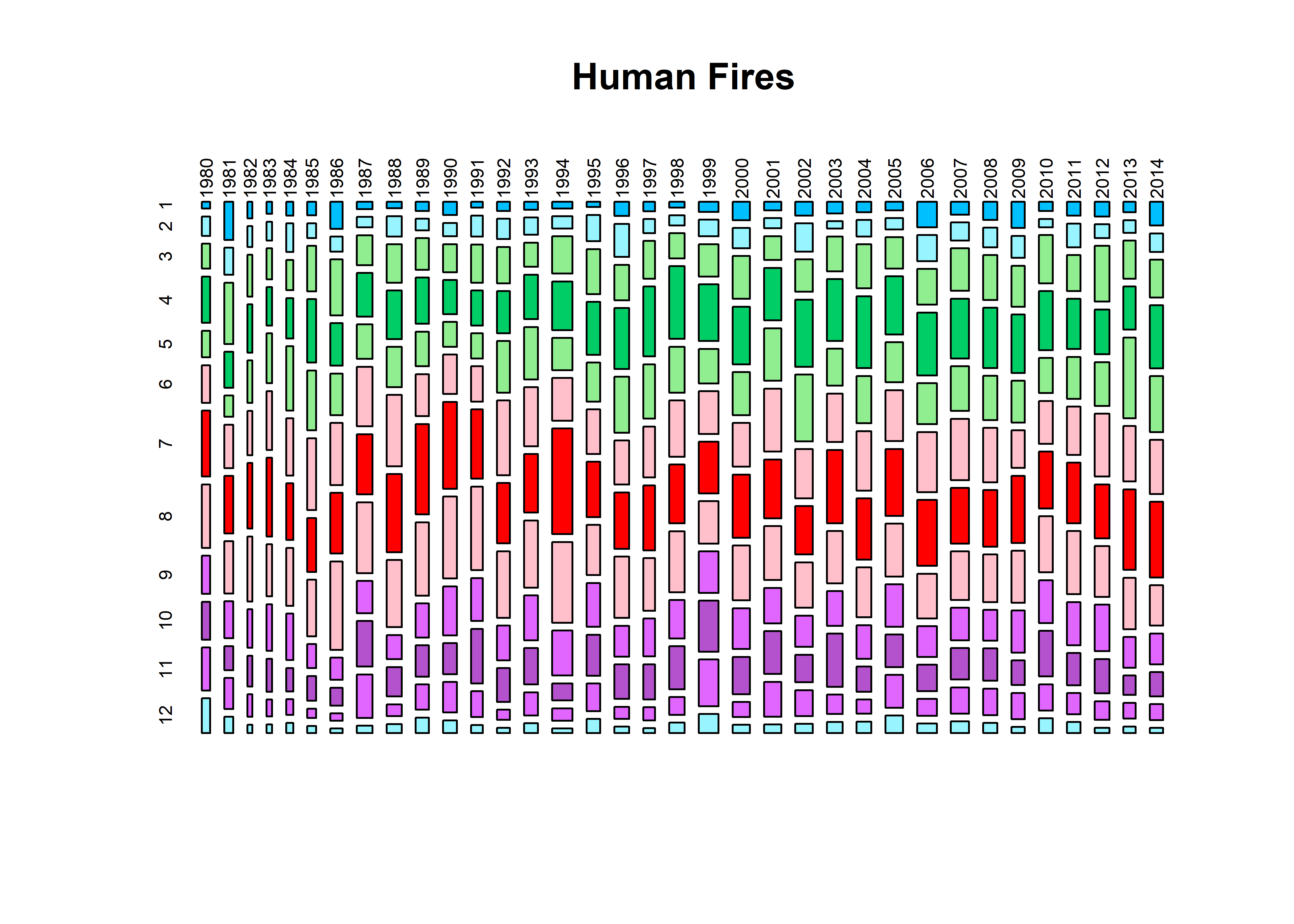
fwfod.tablecause <- table(fwfod$YEAR_, fwfod$ORGANIZATI)
mosaicplot(fwfod.tablecause, cex.axis=0.6, las=3, color=mosaiccolor, main="Fires by Organization")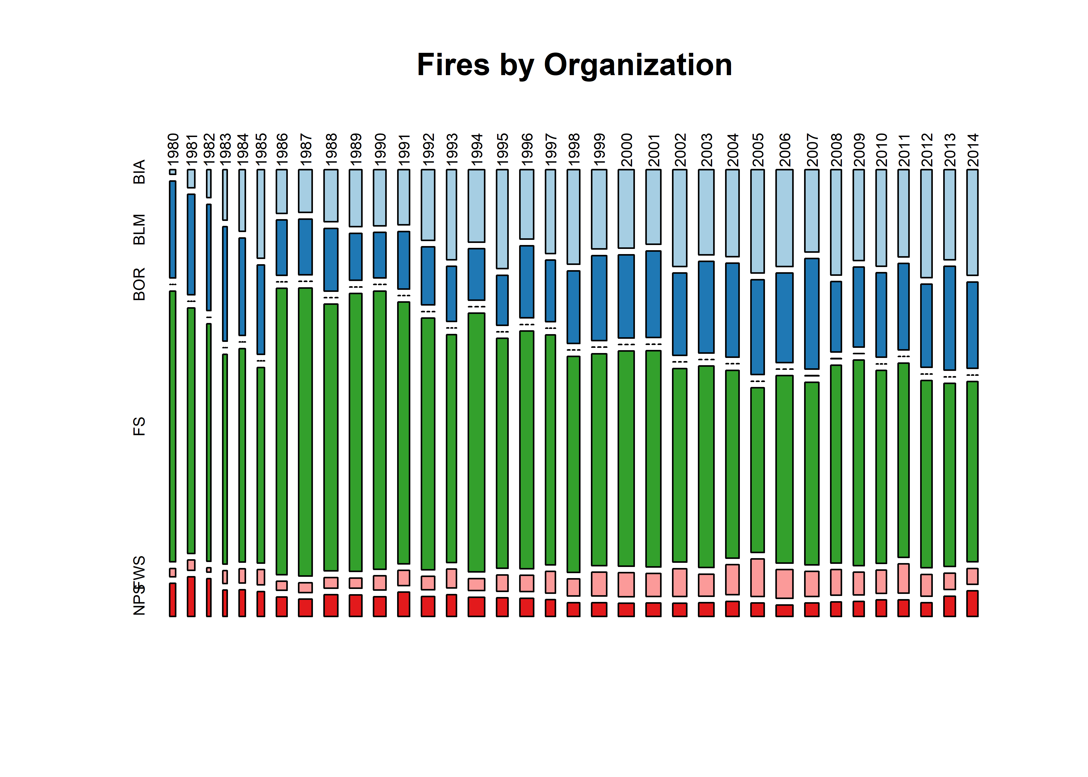
fwfod.tablecause <- table(fwfod$YEAR_, fwfod$CAUSE)
mosaicplot(fwfod.tablecause, cex.axis=0.6, las=3, color=mosaiccolor, main="Fires by Cause")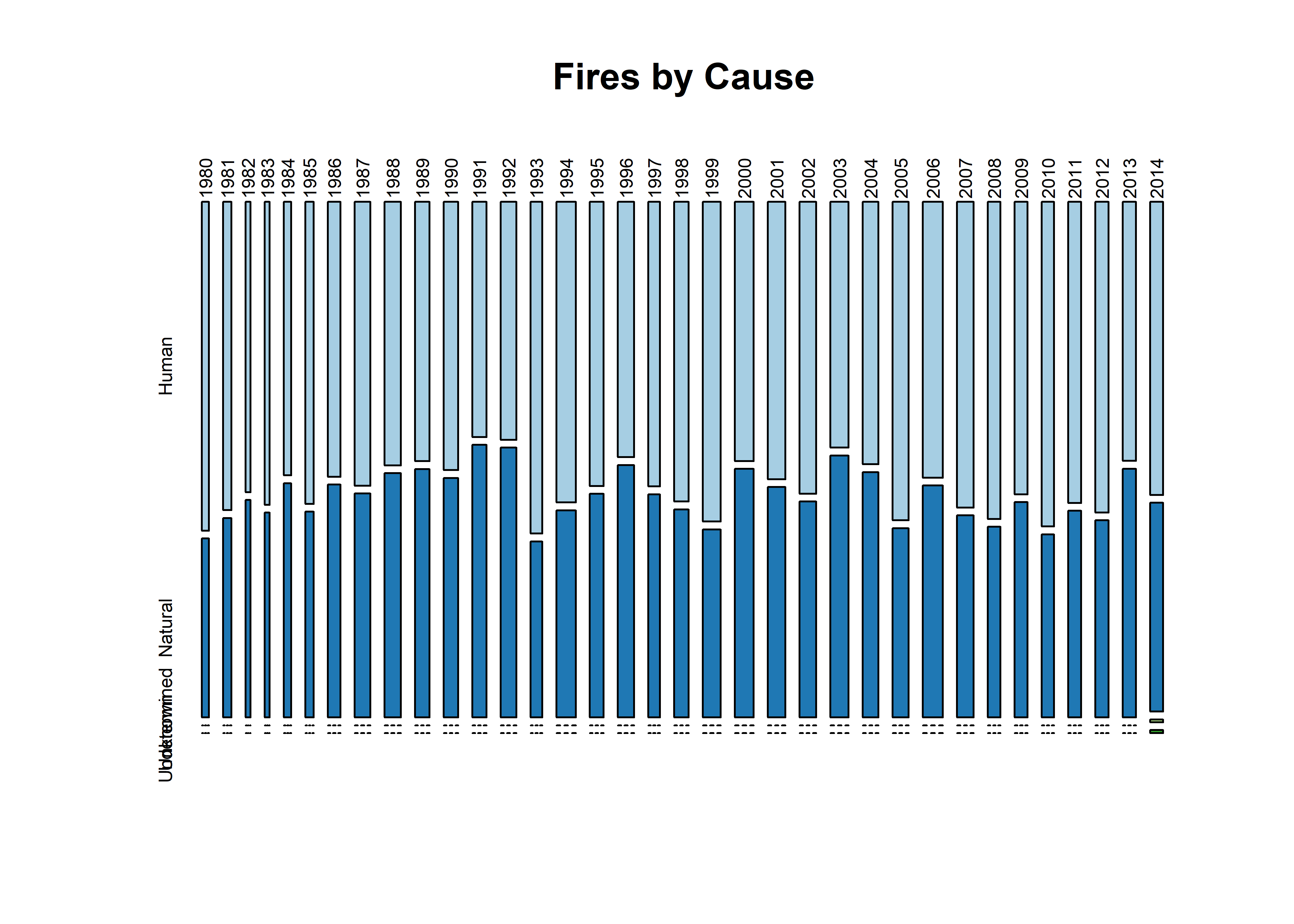
fwfod.tablecause <- table(fwfod$YEAR_, fwfod$STATCAUSE)
mosaicplot(fwfod.tablecause, cex.axis=0.6, las=3, color=mosaiccolor, main="Fires by Cause")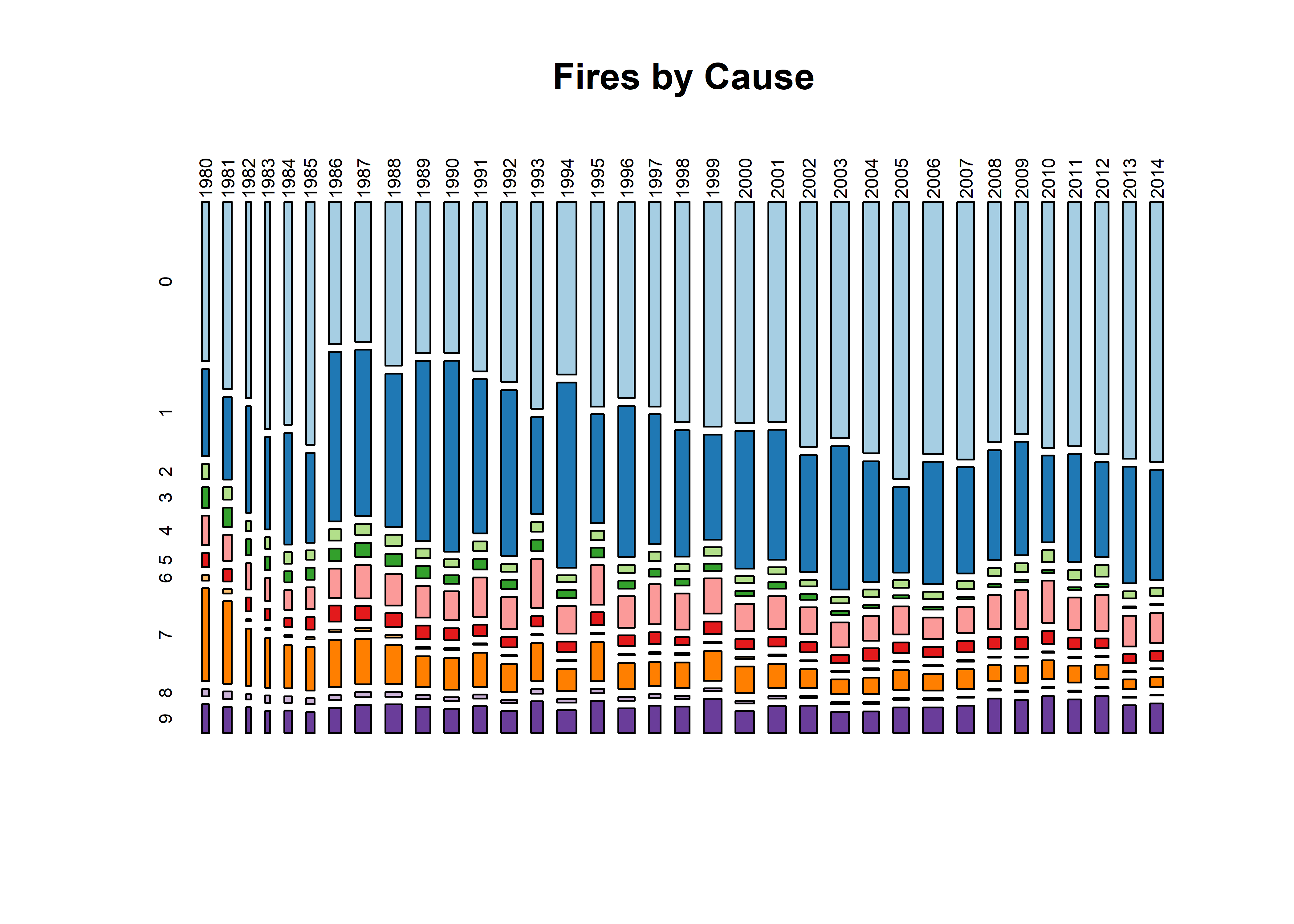
Number of fires/year (FS and FWS)
hist(fwfod$startyear[fwfod$ORGANIZATI=="FS"], xlim=c(1980,2015), ylim=c(0,40000),
  breaks=seq(1979.5,2014.5,by=1))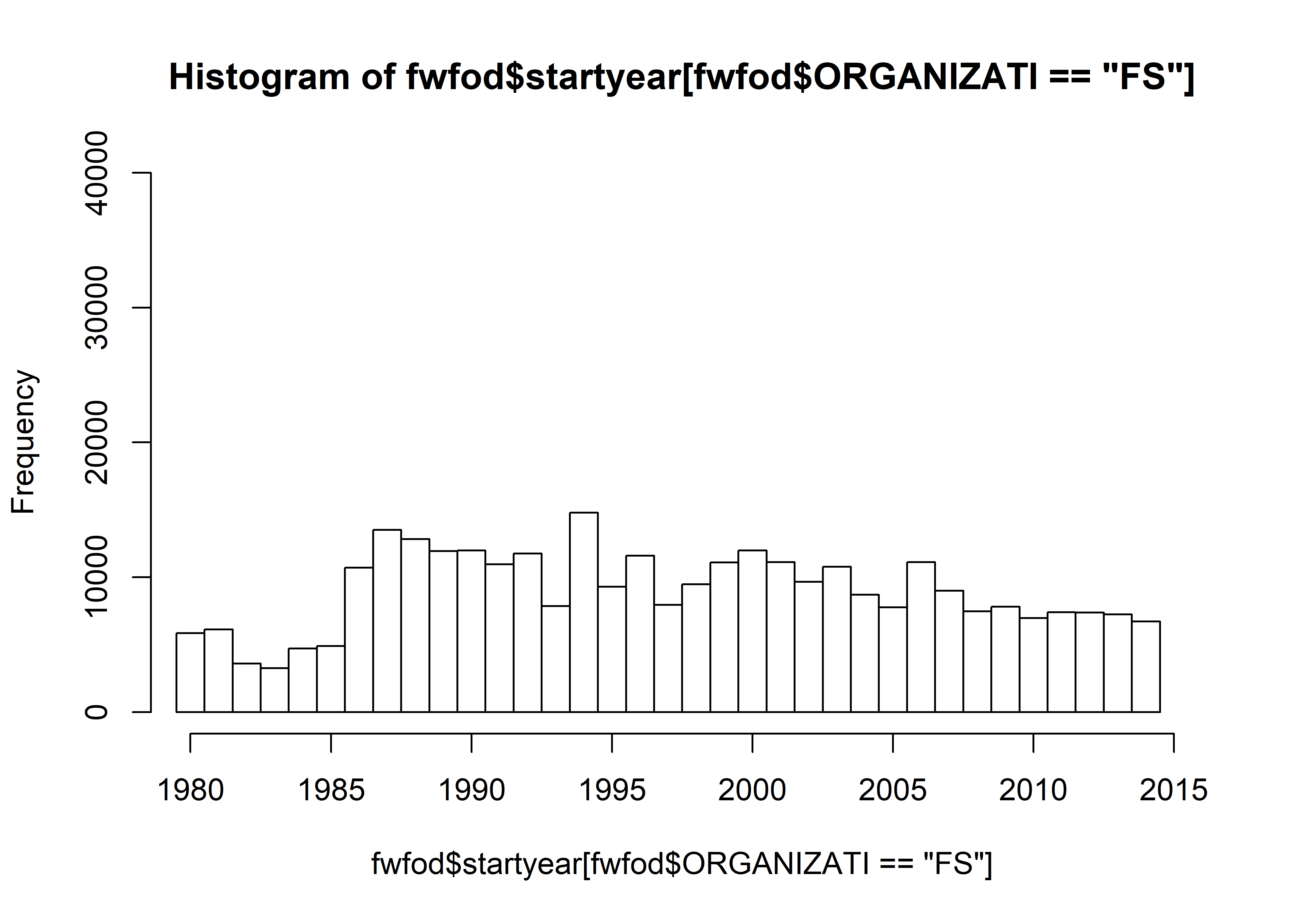
hist(fwfod$startyear[fwfod$ORGANIZATI=="FWS"], xlim=c(1980,2015), ylim=c(0,40000),
  breaks=seq(1979.5,2014.5,by=1))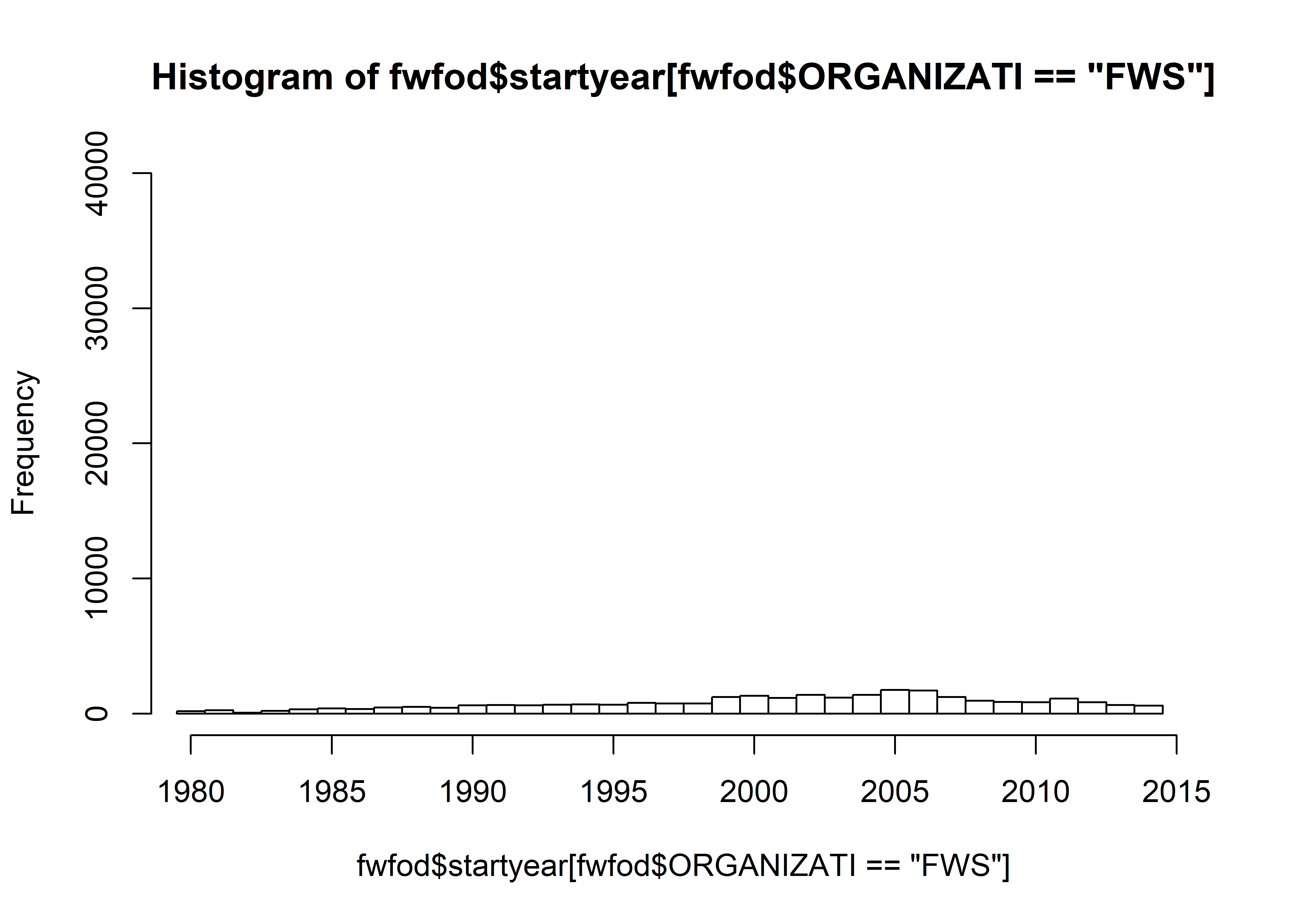
Mosaic plots by agency (FS and FWS)
table(fwfod$ORGANIZATI)##
## BIA BLM BOR FS FWS NPS
## 110079 109759 11 315580 27708 25751fwfod.tablemon <- table(fwfod$YEAR_[fwfod$ORGANIZATI == "FS"],
fwfod$startmon[fwfod$ORGANIZATI == "FS"])
mosaicplot(fwfod.tablemon, color=monthcolors, cex.axis=0.6, las=3, main="All Fires -- FS")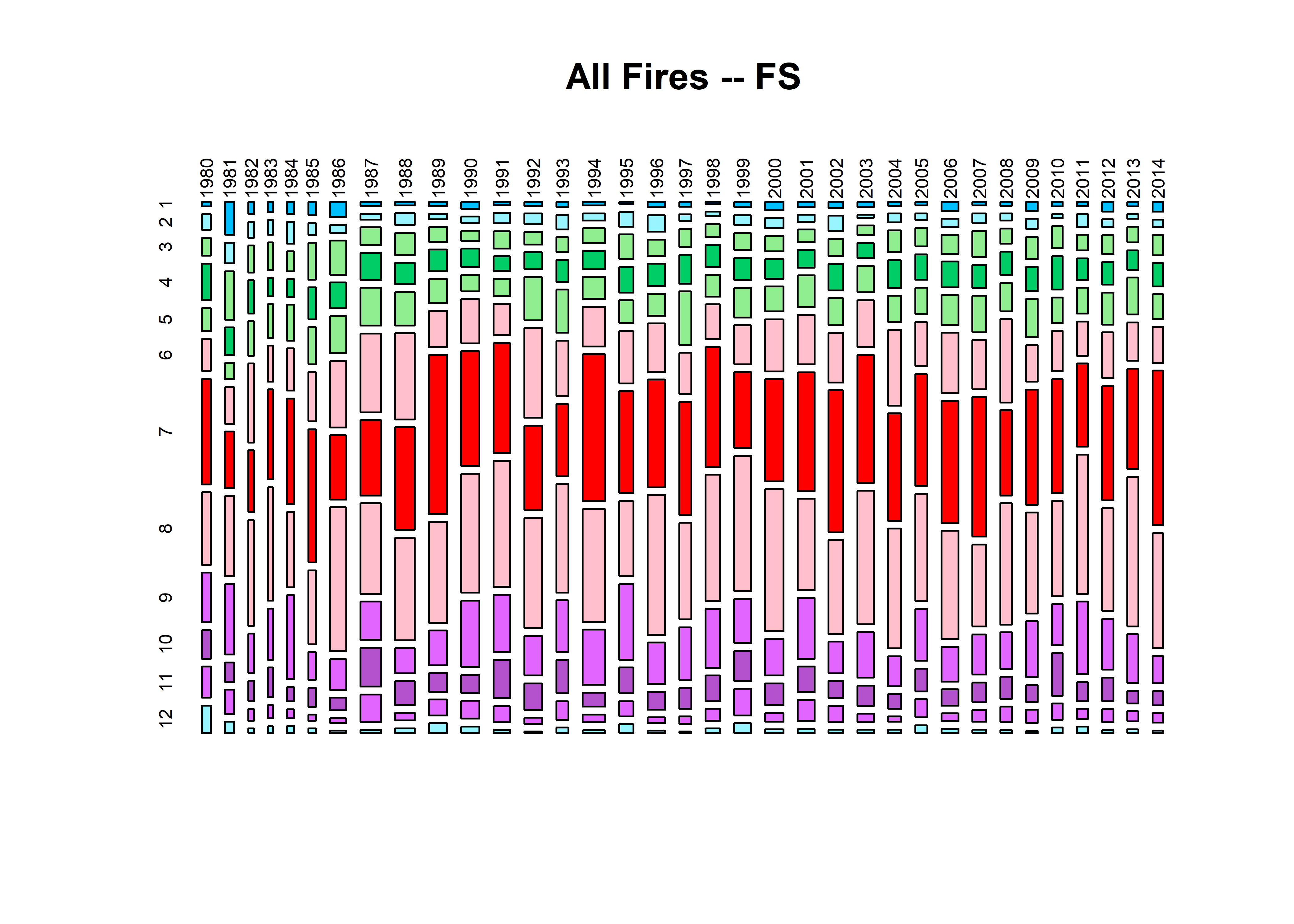
fwfod.tablemon <- table(fwfod$YEAR_[fwfod$ORGANIZATI == "FWS"],
  fwfod$startmon[fwfod$ORGANIZATI == "FWS"])
mosaicplot(fwfod.tablemon, color=monthcolors, cex.axis=0.6, las=3, main="All Fires -- FWS")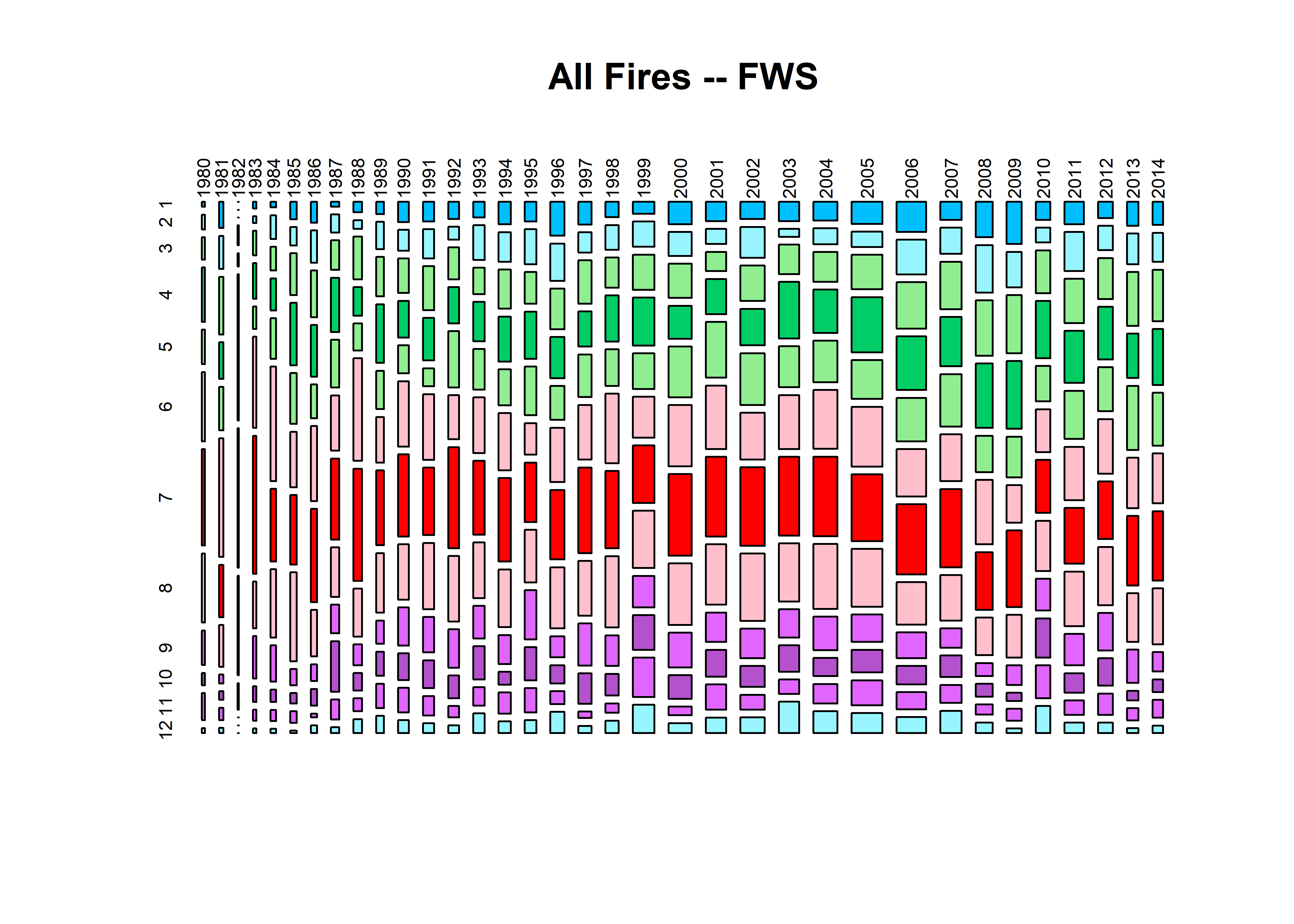
The Forest Service data look well distributed (excepting the potential discontinuities between 1985 and 1986, and between 2007 and 2008). The FWS data (a smaller number of records), looks like there are more discontinuities.
3 Subsets of the FWFOD
3.1 Western U.S. Subset
This subset corresponds to the data set used in Bartlein et al. (2008) (i.e. fires with longitudes <= -102.0)
fwfod.wus <- fwfod[fwfod$DLONGITUDE <= -102.0 & fwfod$DLONGITUDE >= -126.0,]
length(fwfod.wus[,1])
## [1] 450710table(fwfod.wus$CAUSE)##
## Human Natural Undetermined Unknown
## 207675 238889 18 70Map the data
plot(fwfod.wus$DLATITUDE ~ fwfod.wus$DLONGITUDE, ylim=c(27.5,50), xlim=c(-125,-100), type="n",
  xlab="Longitude", ylab="Latitude")
map("world", add=TRUE, lwd=2, col="gray")
map("state", add=TRUE, lwd=2, col="gray")
points(fwfod.wus$DLATITUDE ~ fwfod.wus$DLONGITUDE, pch=16, cex=0.2, col="red")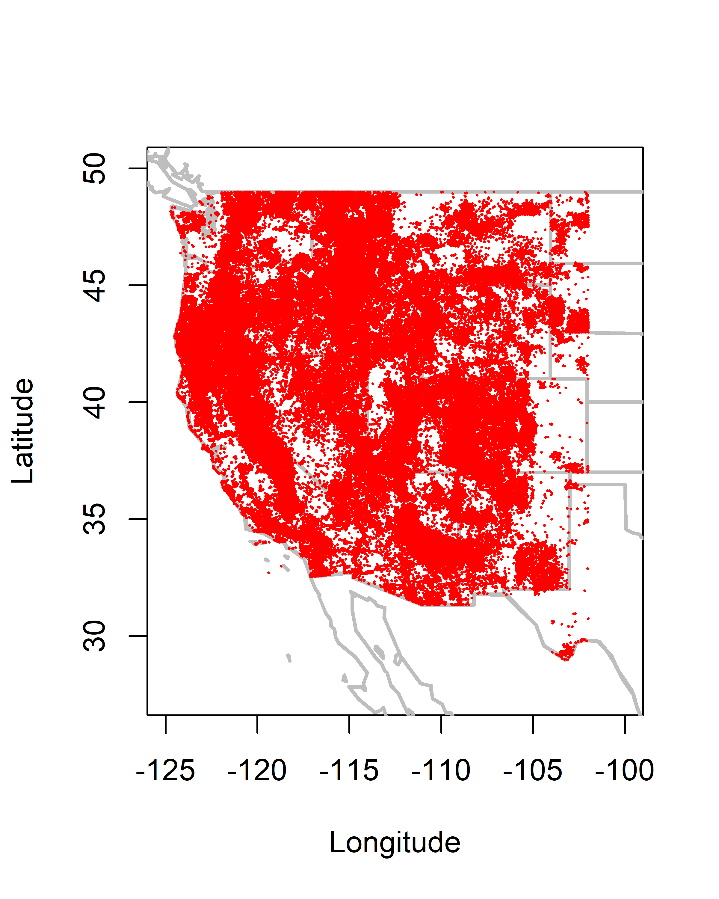
Histograms Western U.S.
hist(fwfod.wus$startdaynum, breaks=seq(-0.5,366.5,by=1), freq=-TRUE, ylim=c(0,6000), xlim=c(0,400))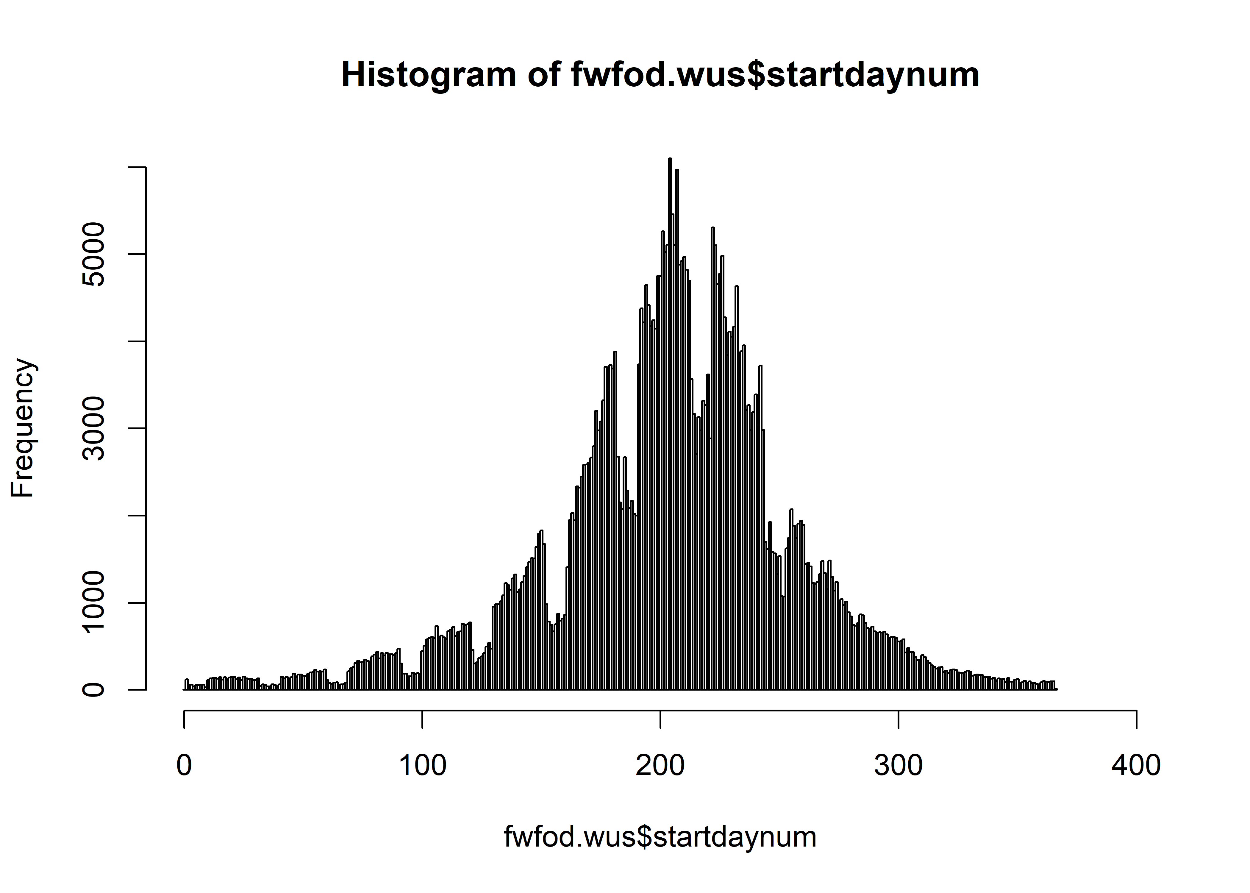
hist(fwfod.wus$startdaynum[fwfod.wus$CAUSE=="Human"], breaks=seq(-0.5,366.5,by=1), freq=-TRUE,
  xlim=c(0,400), ylim=c(0,6000))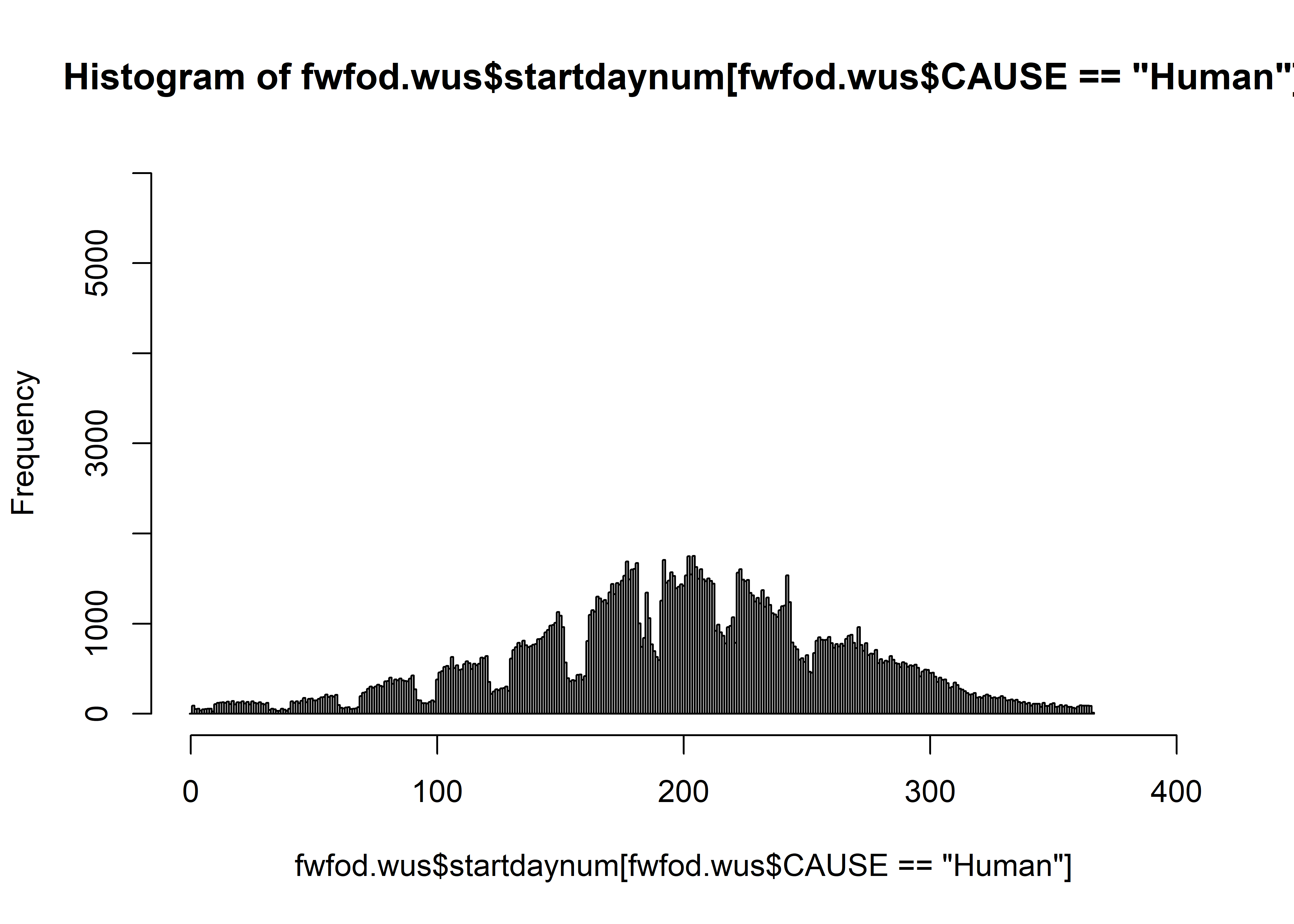
hist(fwfod.wus$startdaynum[fwfod.wus$CAUSE=="Natural"], breaks=seq(-0.5,366.5,by=1), freq=-TRUE,
  xlim=c(0,400), ylim=c(0,6000))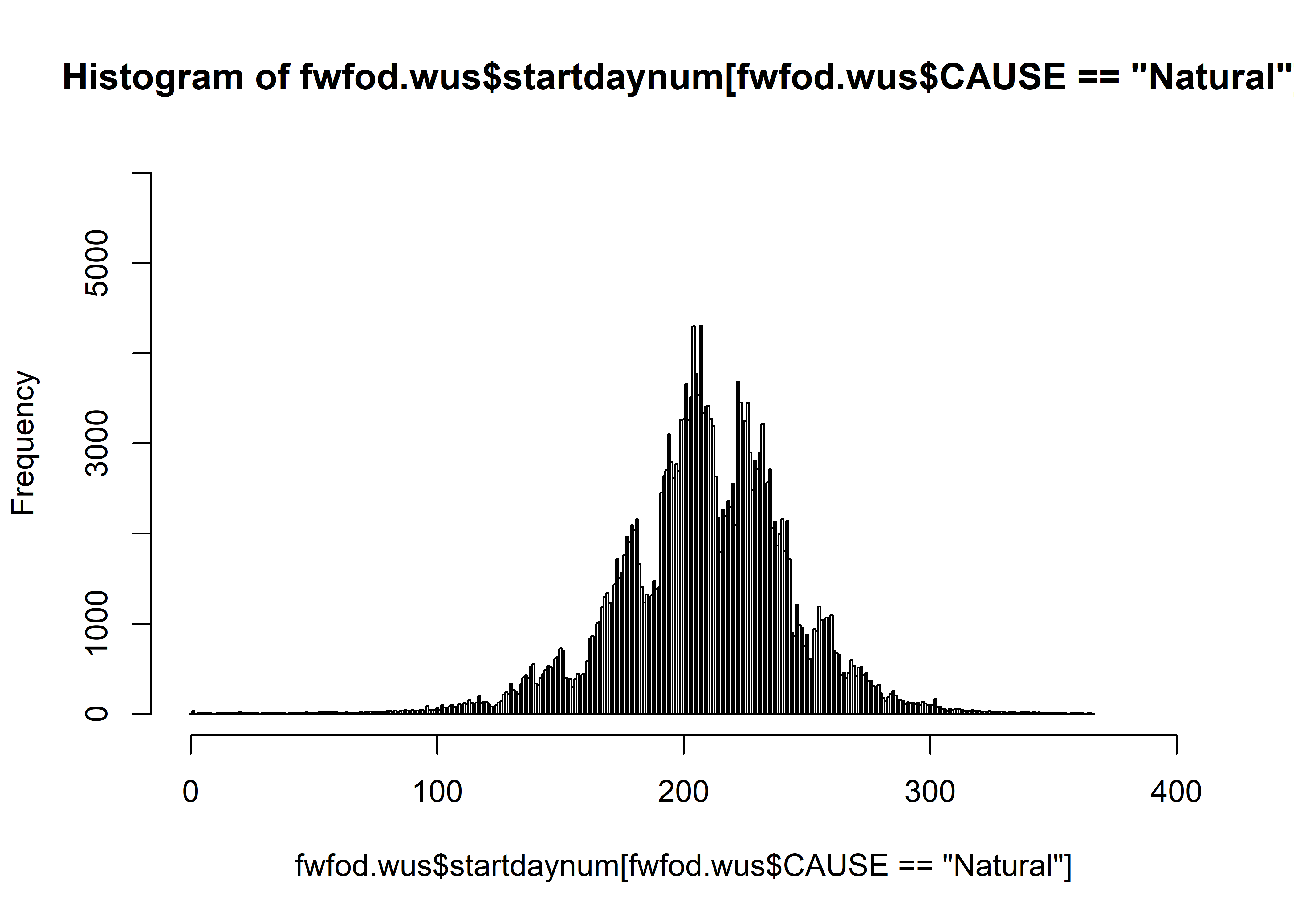
3.2 Alaska Subset
Alaska data
fwfod.ak <- fwfod[fwfod$DLATITUDE >= 55.0 ,]
length(fwfod.ak[,1])
## [1] 8491table(fwfod.ak$CAUSE)##
## Human Natural Undetermined Unknown
## 2947 5174 1 3Map the data
plot(fwfod.ak$DLATITUDE ~ fwfod.ak$DLONGITUDE, ylim=c(50,80), xlim=c(-180,-125), type="n",
  xlab="Longitude", ylab="Latitude")
map("world", add=TRUE, lwd=2, col="gray")
map("state", add=TRUE, lwd=2, col="gray")
points(fwfod.ak$DLATITUDE ~ fwfod.ak$DLONGITUDE, pch=16, cex=0.2, col="red")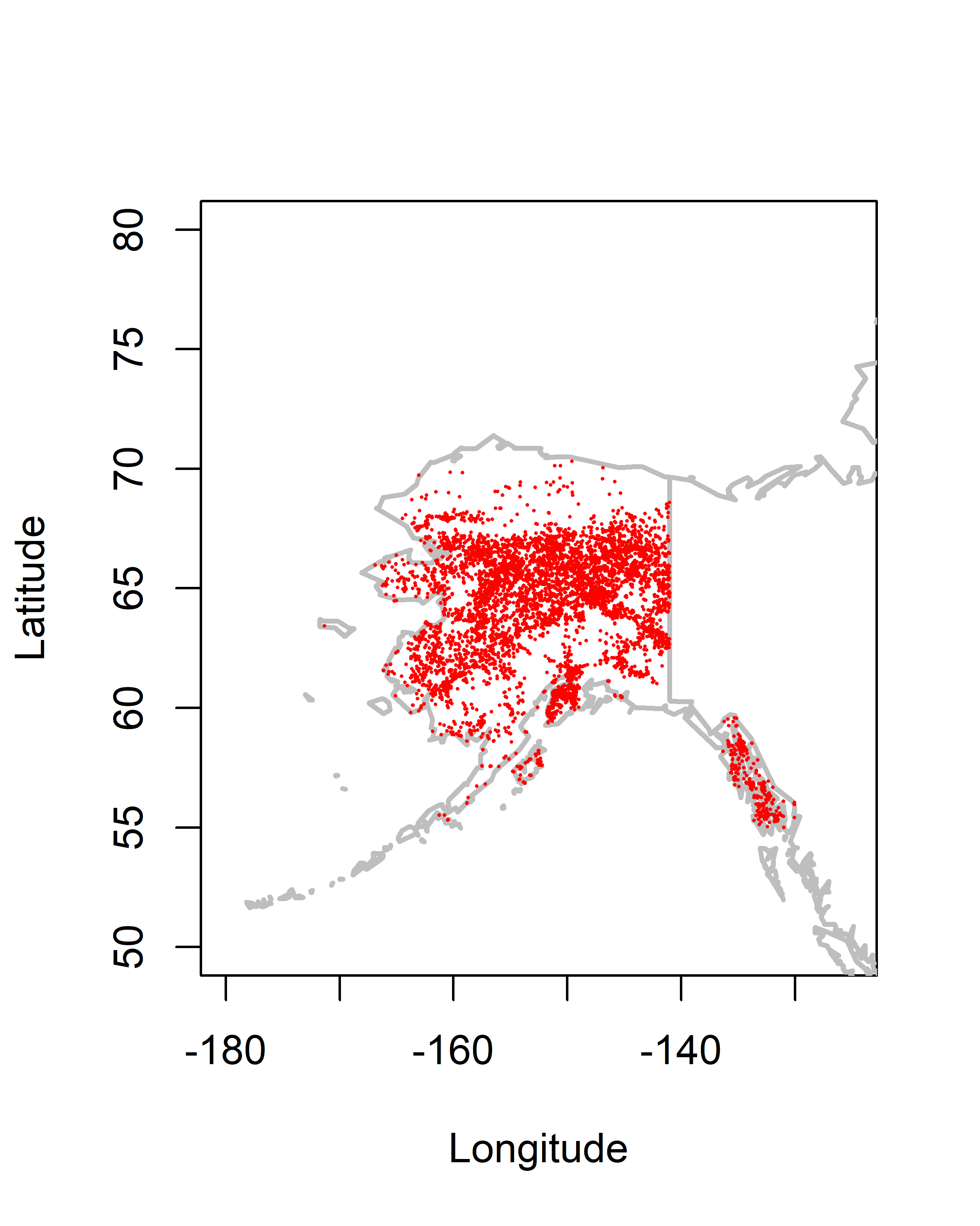
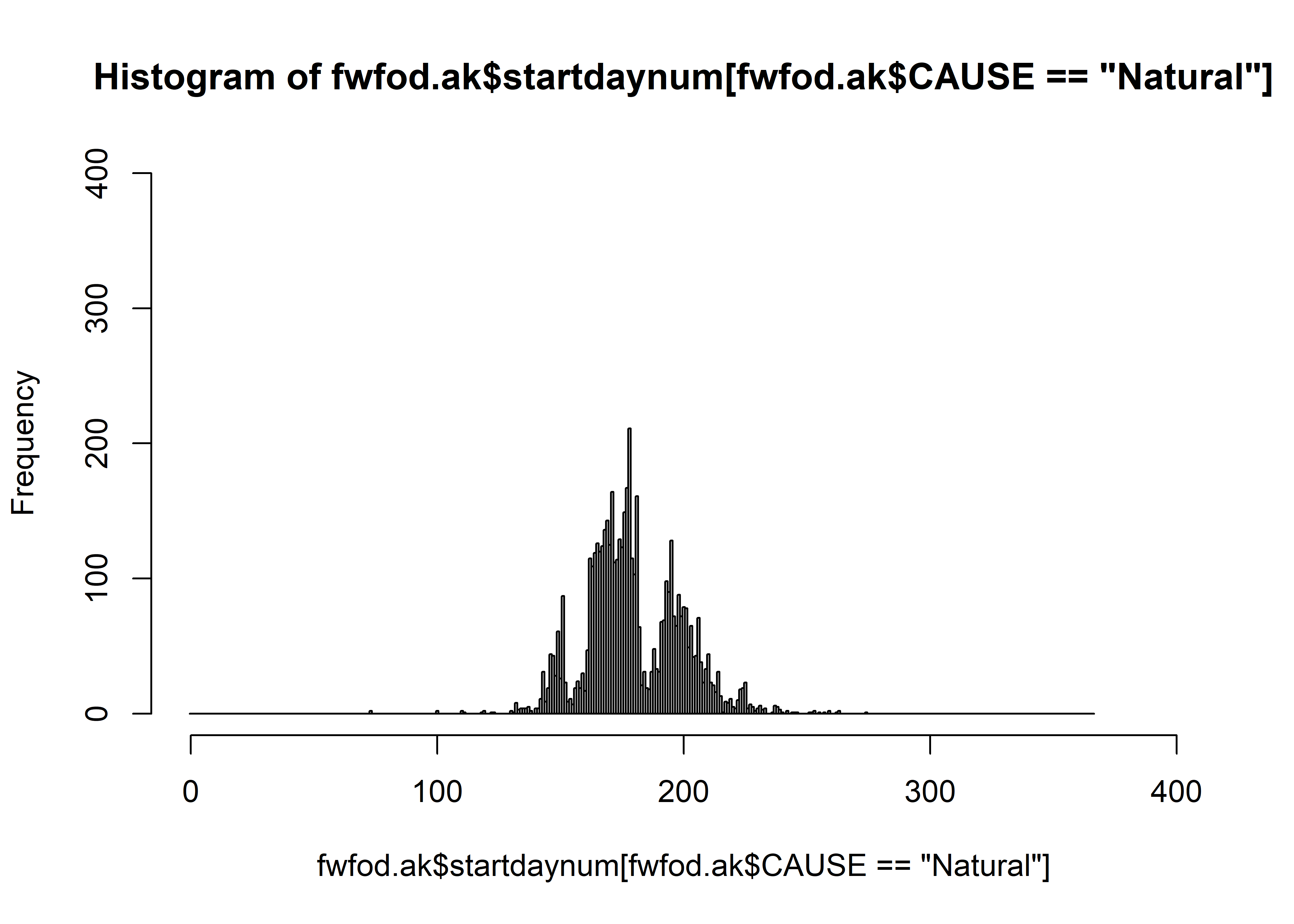
Histograms Alaska
hist(fwfod.ak$startdaynum, breaks=seq(-0.5,366.5,by=1), freq=-TRUE, ylim=c(0,400), xlim=c(0,400))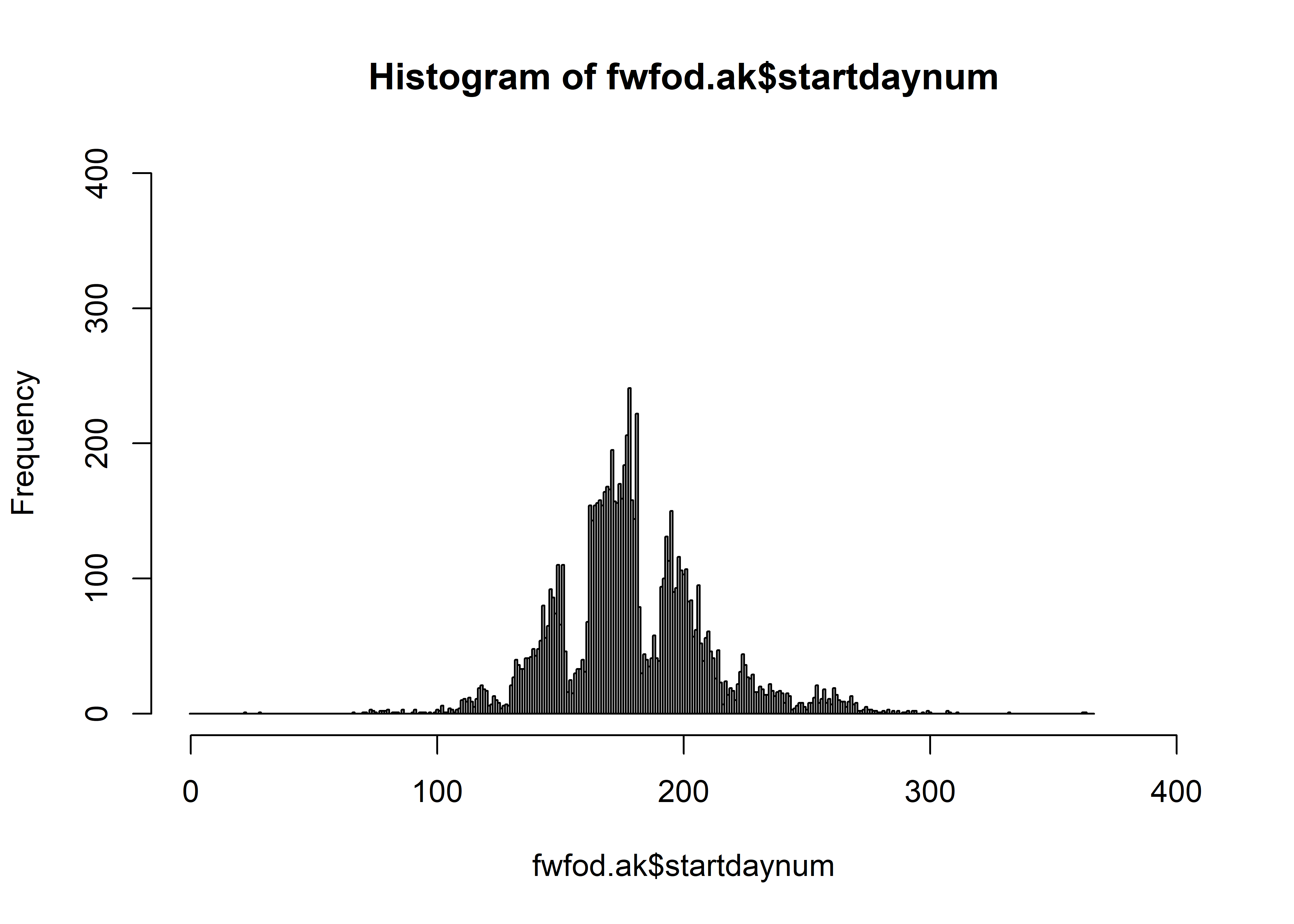
hist(fwfod.ak$startdaynum[fwfod.ak$CAUSE=="Human"], breaks=seq(-0.5,366.5,by=1), freq=-TRUE,
  xlim=c(0,400), ylim=c(0,400))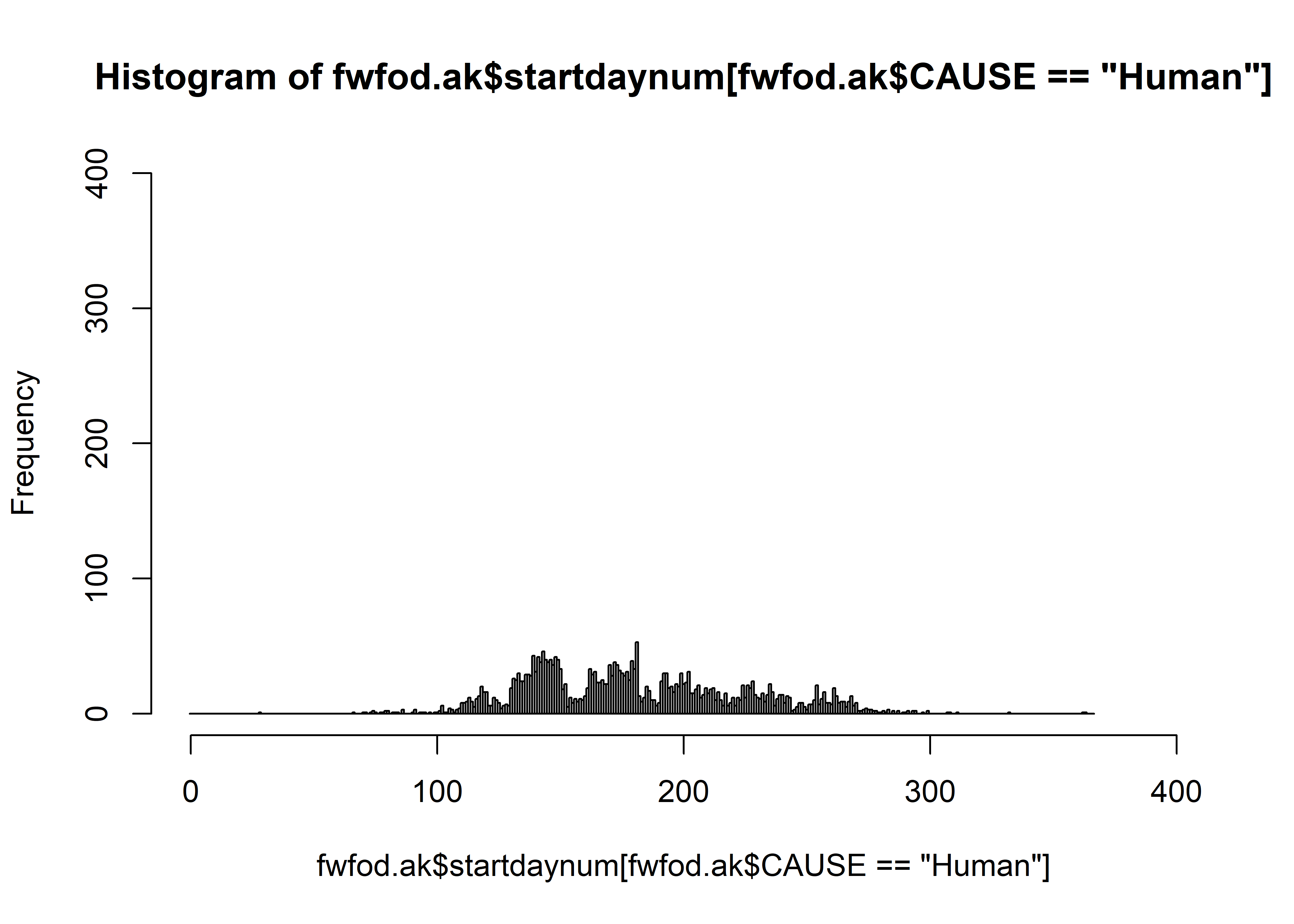
hist(fwfod.ak$startdaynum[fwfod.ak$CAUSE=="Natural"], breaks=seq(-0.5,366.5,by=1), freq=-TRUE,
  xlim=c(0,400), ylim=c(0,400))