Size-distributions of US & Canada merged data
1 Analysis of the size distributions of lightning-started fires
1.1 Overview
The U.S. and Candadian data sets are observed with different area units – acres and hectares, respectively – and so might be expected to be non-homogeneous, or structurally different, at small fire sizes. Here we analyze the size-distribution of the two data sets, separately and jointly, and restricted to lightning-started fires, to avoid the further complication of natural-vs-human ignitions, in order to determine the extent of that non-homogenetity and to identify a minimum-size threshold that can be used to reduce the “noice” of small fire sizes.
1.2 Lightning fire numbers and sizes
load the merged data set
load("e:/Projects/fire/DailyFireStarts/data/RData/uscan_1986-2013.RData")1.2.1 US (FPA-FOD data)
Get FPA-FOD data:
fpafod <- uscan[uscan$datasource == "fpafod", ]Get lightning fires. The folowing code 1) gets the fires, 2) filters by cause, 3) sorts the data from smallest to largest fire.
# get lighting-only fires
fpafod.lt <- fpafod[fpafod$cause1 == 1 ,]
fpafod.nfires <- length(fpafod.lt[,1])
fpafod.nfires
## [1] 260311fpafod.index <-order(fpafod.lt$area_ha, na.last=FALSE)
fpafod.lt <- fpafod.lt[fpafod.index ,]
fpafod.lt$rank <- seq(fpafod.nfires, 1)
head(cbind(fpafod.lt$area_ha,fpafod.lt$rank))## [,1] [,2]
## [1,] 0.0000404686 260311
## [2,] 0.0000404686 260310
## [3,] 0.0000809372 260309
## [4,] 0.0001857509 260308
## [5,] 0.0004046860 260307
## [6,] 0.0004046860 260306tail(cbind(fpafod.lt$area_ha,fpafod.lt$rank))## [,1] [,2]
## [260306,] 195576.7 6
## [260307,] 202320.7 5
## [260308,] 209254.2 4
## [260309,] 217570.1 3
## [260310,] 225895.0 2
## [260311,] 245622.1 1Write a .csv files for browsing in Excel
csvpath="e:/Projects/fire/DailyFireStarts/data/MergedData/"
write.table(fpafod.lt, paste(csvpath,"fpafod.lt.csv", sep=""), row.names=FALSE, sep=",")
Save the R dataset
outworkspace="fpafod.lt.RData"
save.image(file=outworkspace)
1.2.2 Canada (CNFDB)
Get CNFDB data:
cnfdb <- uscan[uscan$datasource == "cnfdb", ]Get lightning fires. The folowing code 1) gets the fires, 2) filters by cause, 3) sorts the data from smallest to largest fire.
# get lighting-only fires
cnfdb.lt <- cnfdb[cnfdb$cause1 == 1 ,]
cnfdb.nfires <- length(cnfdb.lt[,1])
cnfdb.nfires
## [1] 99041cnfdb.index <-order(cnfdb.lt$area_ha, na.last=FALSE)
cnfdb.lt <- cnfdb.lt[cnfdb.index ,]
cnfdb.lt$rank <- seq(cnfdb.nfires, 1)
head(cbind(cnfdb.lt$area_ha,cnfdb.lt$rank))## [,1] [,2]
## [1,] 0 99041
## [2,] 0 99040
## [3,] 0 99039
## [4,] 0 99038
## [5,] 0 99037
## [6,] 0 99036tail(cbind(cnfdb.lt$area_ha,cnfdb.lt$rank))## [,1] [,2]
## [99036,] 428100.0 6
## [99037,] 438000.0 5
## [99038,] 453144.0 4
## [99039,] 466420.3 3
## [99040,] 501689.1 2
## [99041,] 553680.0 1Write a .csv files for browsing in Excel
csvpath="e:/Projects/fire/DailyFireStarts/data/MergedData/"
write.table(cnfdb.lt, paste(csvpath,"cnfdb.lt.csv", sep=""), row.names=FALSE, sep=",")
Save the R dataset
outworkspace="cnfdb.lt.RData"
save.image(file=outworkspace)
2 Spatial patterns
There are two basic views of the two data sets that suggest that (in addition to issues like zero-area fires), that the data sets cannot be casually merged. These are 1) the map patterns, and 2 the (size and number) distributions (i.e. histograms) of the data.
2.1 Map patterns
library(maps)
options(width=110)
Map the location of all fires
plot(0,0, ylim=c(17,80), xlim=c(-180,-55), type="n",
  xlab="longitude", ylab="latitude", main="All Lightning Fires")
map("world", add=TRUE, lwd=2, col="gray")
points(cnfdb.lt$latitude ~ cnfdb.lt$longitude, pch=16, cex=0.3, col="red")
points(fpafod.lt$latitude ~ fpafod.lt$longitude, pch=16, cex=0.3, col="red")
There are some obvious artifacts in the spatial patterns.
2.1.1 NY and adjacent regions
New York stands out, especially Long Is.:
plot(0,0, ylim=c(40,55), xlim=c(-100,-60), type="n",
  xlab="longitude", ylab="latitude", main="All Lightning Fires")
map(c("world"), add=TRUE, lwd=2, col="gray")
map(c("state"), add=TRUE, lwd=2, col="gray")
points(cnfdb.lt$latitude ~ cnfdb.lt$longitude, pch=16, cex=0.3, col="red")
points(fpafod.lt$latitude ~ fpafod.lt$longitude, pch=16, cex=0.3, col="red")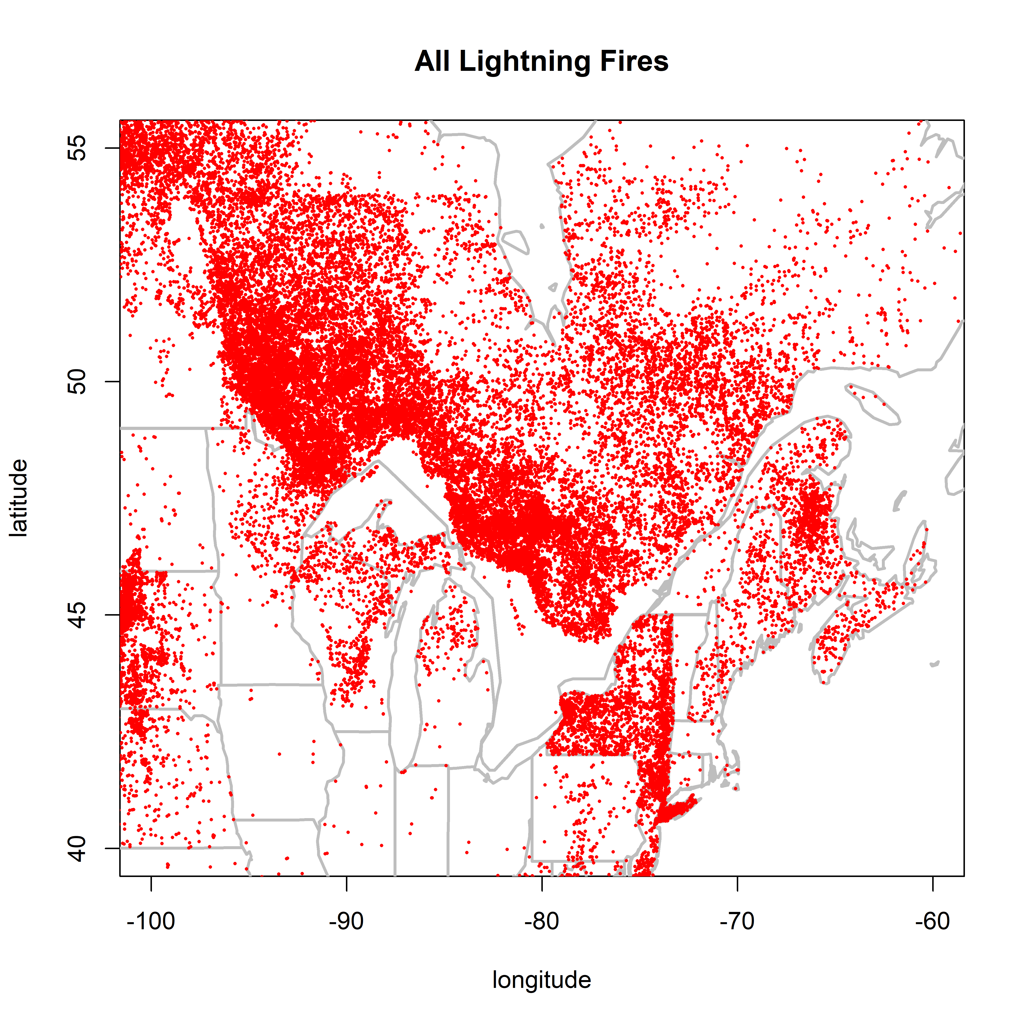
2.1.2 Great Plains
There seem to be very frew lightning fires in Kansas. There are some good things, however, in particular the prairie-forest border in Manitoba and Minnesota.
plot(0,0, ylim=c(30,55), xlim=c(-115,-90), type="n",
  xlab="longitude", ylab="latitude", main="All Lightning Fires")
map(c("world"), add=TRUE, lwd=2, col="gray")
map(c("state"), add=TRUE, lwd=2, col="gray")
points(cnfdb.lt$latitude ~ cnfdb.lt$longitude, pch=16, cex=0.3, col="red")
points(fpafod.lt$latitude ~ fpafod.lt$longitude, pch=16, cex=0.3, col="red")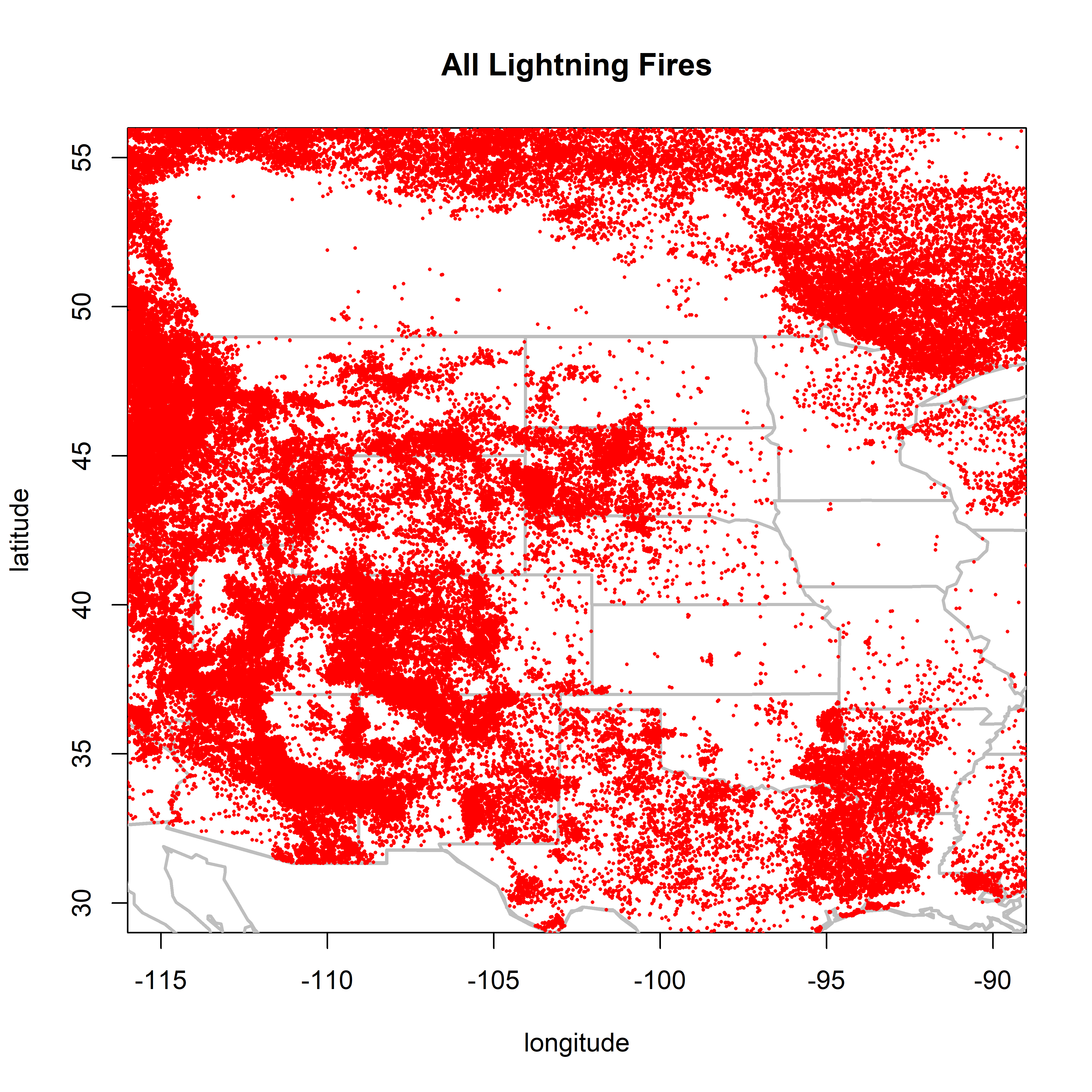
2.1.3 PNW
PNW Looks ok–no sign of country-border discontinuity.
plot(0,0, ylim=c(40,55), xlim=c(-130,-105), type="n",
  xlab="longitude", ylab="latitude", main="All Lightning Fires")
map("world", add=TRUE, lwd=2, col="gray")
map(c("state"), add=TRUE, lwd=2, col="gray")
points(cnfdb.lt$latitude ~ cnfdb.lt$longitude, pch=16, cex=0.3, col="red")
points(fpafod.lt$latitude ~ fpafod.lt$longitude, pch=16, cex=0.3, col="red")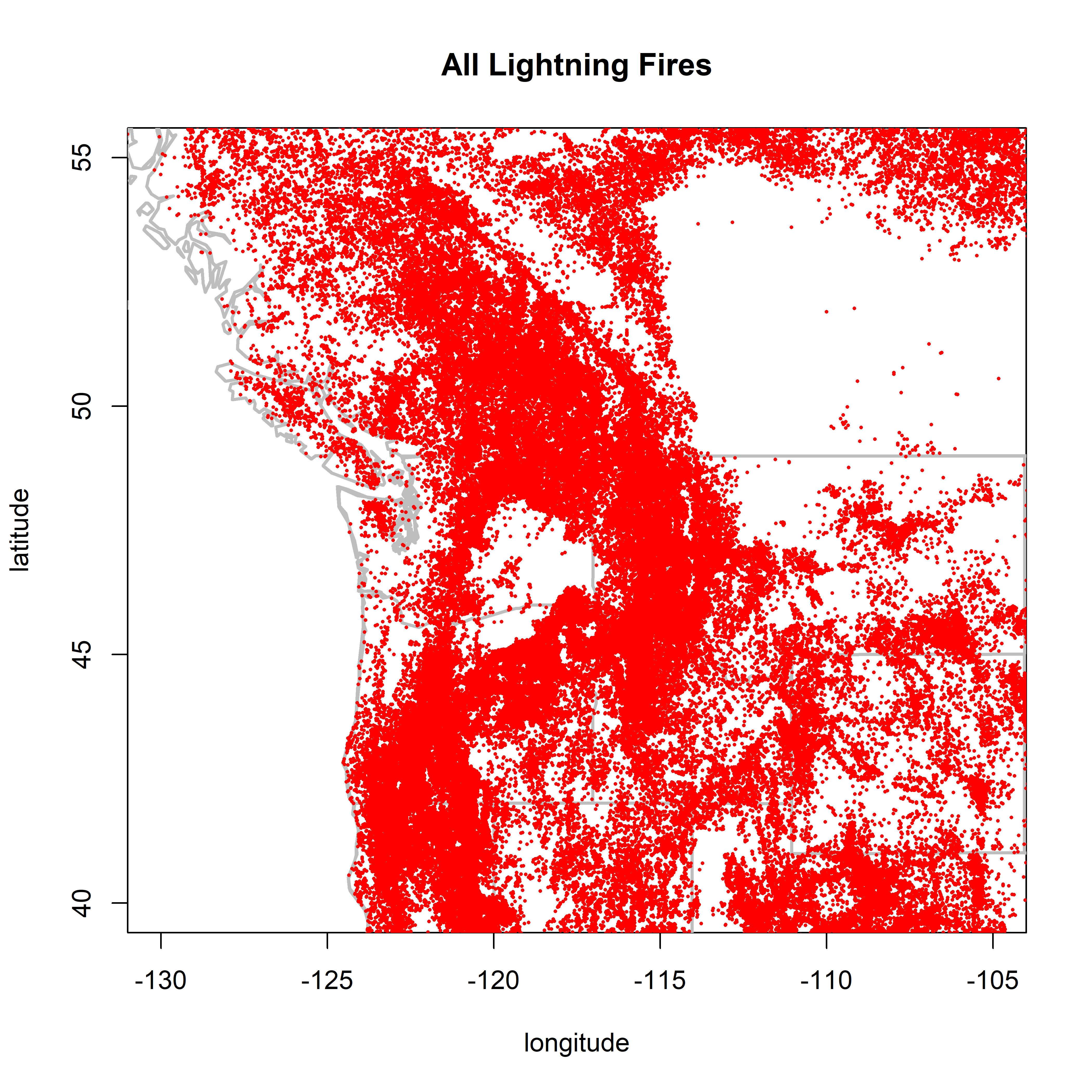
2.1.4 AK/NW Canada
There is a hint of a little discontinuity between Alaska and Canada.
plot(0,0, ylim=c(55,70), xlim=c(-165,-135), type="n",
  xlab="longitude", ylab="latitude", main="All Lightning Fires")
map("world", add=TRUE, lwd=2, col="gray")
points(cnfdb.lt$latitude ~ cnfdb.lt$longitude, pch=16, cex=0.3, col="red")
points(fpafod.lt$latitude ~ fpafod.lt$longitude, pch=16, cex=0.3, col="red")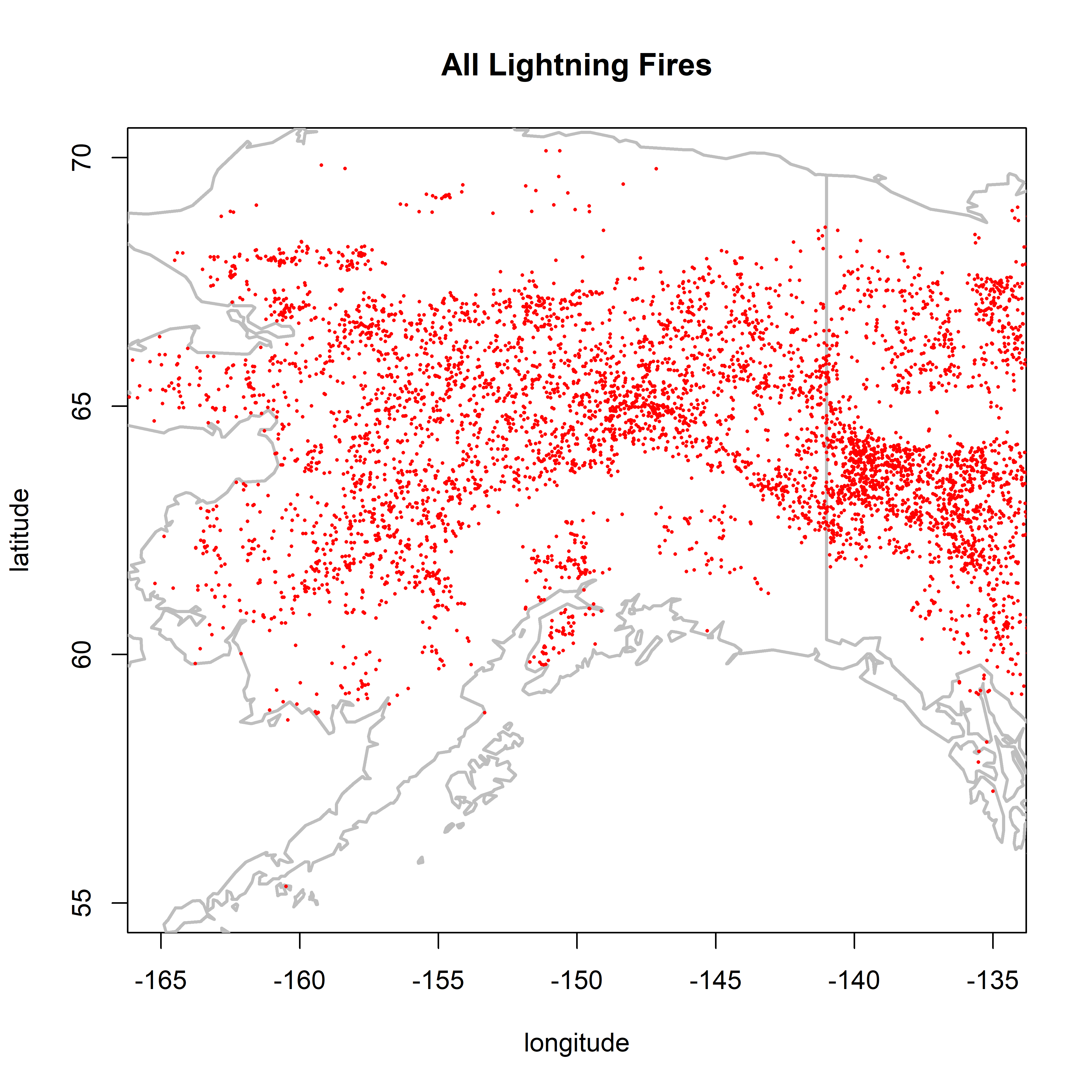
2.2 Map patterns by size class
2.2.1 Fires larger than 0.5 ha
cutsize <- 0.5
plot(0,0, ylim=c(17,80), xlim=c(-180,-55), type="n",
  xlab="longitude", ylab="latitude", main=paste("All Lightning Fires >",as.character(cutsize),"ha"))
map("world", add=TRUE, lwd=2, col="gray")
points(cnfdb.lt$latitude[cnfdb.lt$area_ha >= cutsize] ~ cnfdb.lt$longitude[cnfdb.lt$area_ha >= cutsize],
  pch=16, cex=0.3, col="red")
points(fpafod.lt$latitude[fpafod.lt$area_ha >= cutsize] ~ fpafod.lt$longitude[fpafod.lt$area_ha >= cutsize],
  pch=16, cex=0.3, col="red")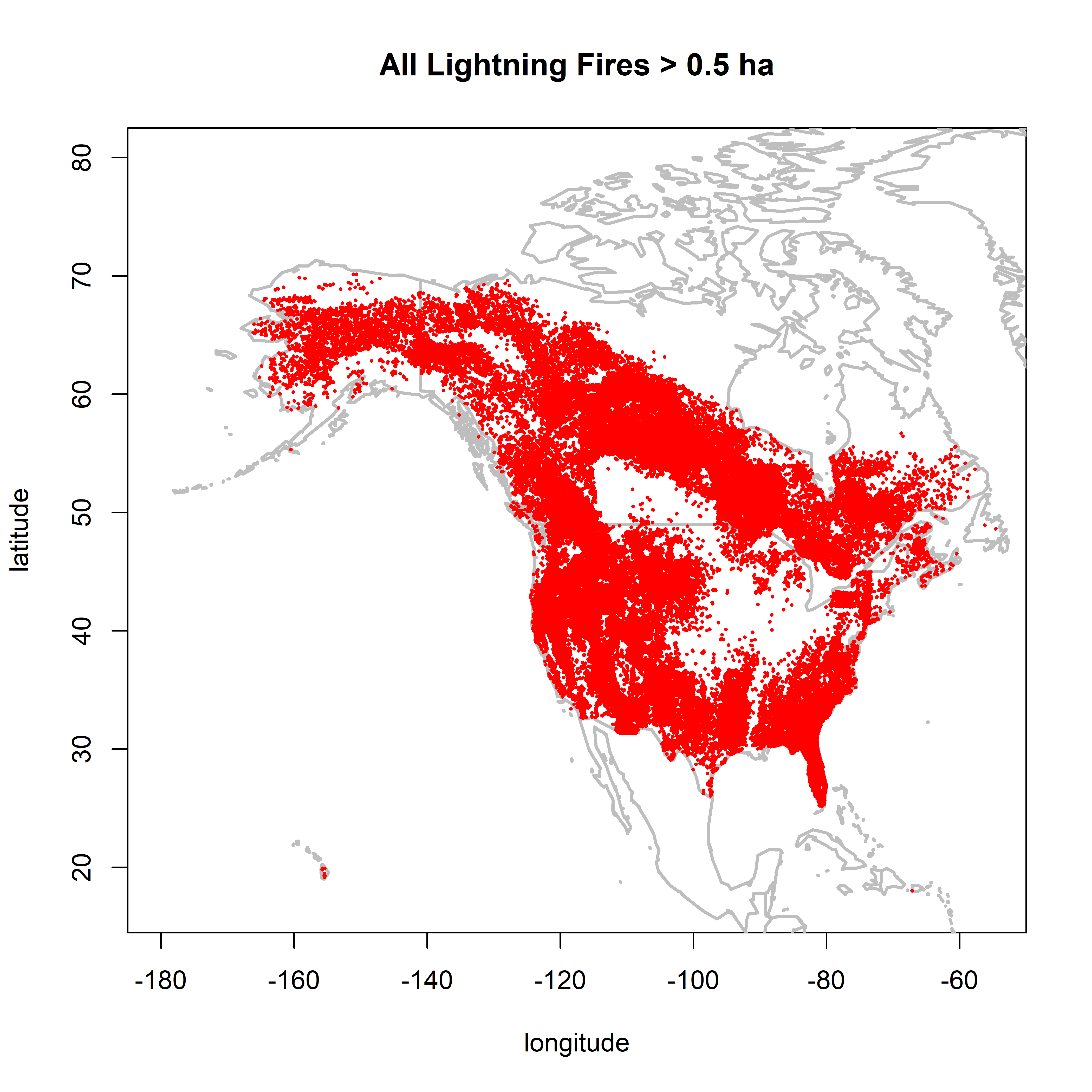
2.2.2 Fires larger than 1.0 ha
cutsize <- 1.0
plot(0,0, ylim=c(17,80), xlim=c(-180,-55), type="n",
  xlab="longitude", ylab="latitude", main=paste("All Lightning Fires >",as.character(cutsize),"ha"))
map("world", add=TRUE, lwd=2, col="gray")
points(cnfdb.lt$latitude[cnfdb.lt$area_ha >= cutsize] ~ cnfdb.lt$longitude[cnfdb.lt$area_ha >= cutsize],
  pch=16, cex=0.3, col="red")
points(fpafod.lt$latitude[fpafod.lt$area_ha >= cutsize] ~ fpafod.lt$longitude[fpafod.lt$area_ha >= cutsize],
  pch=16, cex=0.3, col="red")
2.2.3 Fires larger than 10.0 ha
cutsize <- 10.0
plot(0,0, ylim=c(17,80), xlim=c(-180,-55), type="n",
  xlab="longitude", ylab="latitude", main=paste("All Lightning Fires >",as.character(cutsize),"ha"))
map("world", add=TRUE, lwd=2, col="gray")
points(cnfdb.lt$latitude[cnfdb.lt$area_ha >= cutsize] ~ cnfdb.lt$longitude[cnfdb.lt$area_ha >= cutsize],
  pch=16, cex=0.3, col="red")
points(fpafod.lt$latitude[fpafod.lt$area_ha >= cutsize] ~ fpafod.lt$longitude[fpafod.lt$area_ha >= cutsize],
  pch=16, cex=0.3, col="red")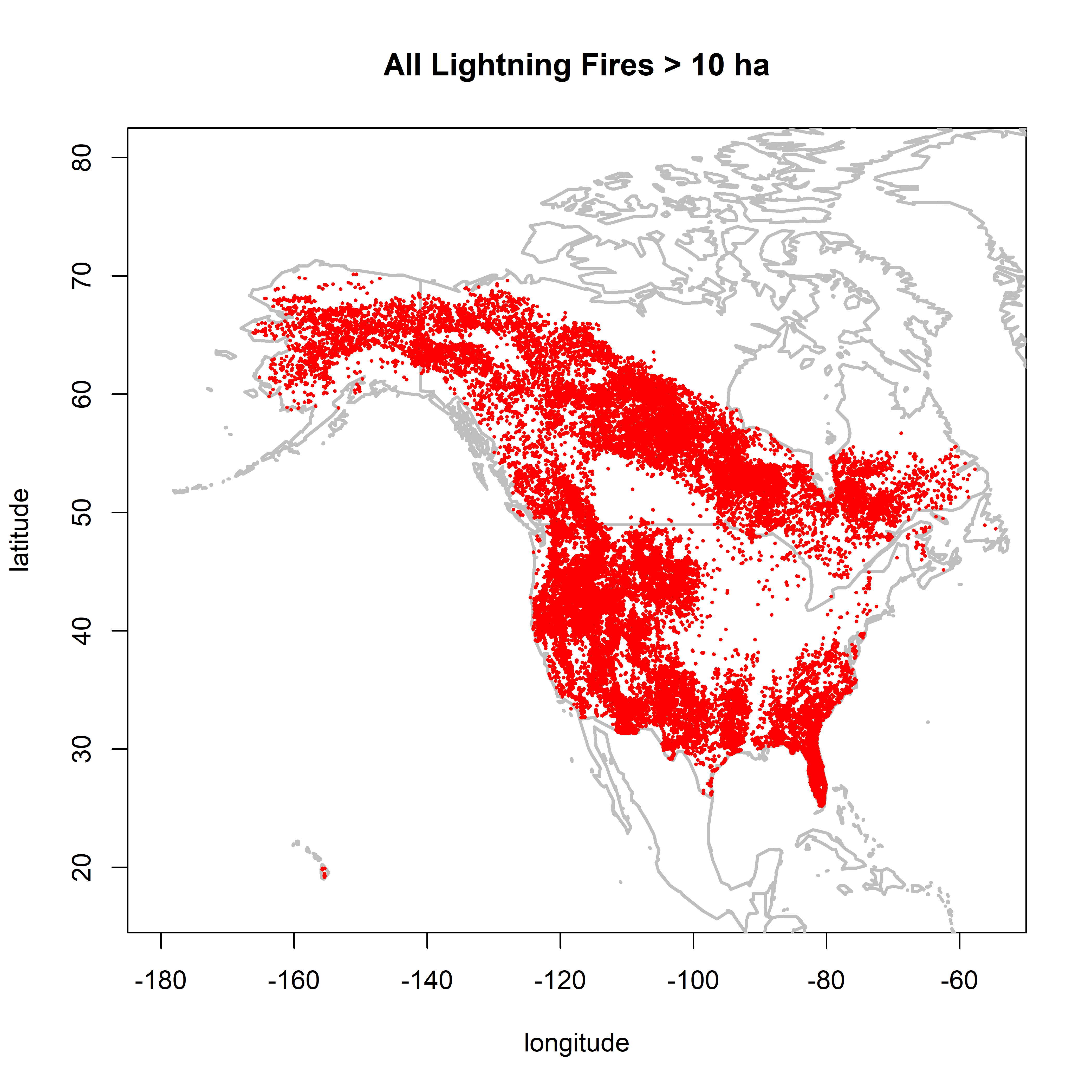
There is little difference in the patterns between 0.5 and 1.0 ha, but the NY overrepresentation issue is much reduced. Between 1.0 and 10.0 ha, the overall number of points are naturally reduced, but the overall patterns remain.
3 Size distributions
3.1 Simple histograms
The idea here is to look at the distributions (e.g. histograms) of the two data sets. It’s going to turn out that the differ quite a bit. There are two possible reasons for that outcome: 1) they differ becauses of unavoidable/unfixable difference in the way the data were collected, or 2) they differ owing to the different environments of Canada and the U.S. (including Alaska). It will also turn out that the distributions at the low end of the range of fire sizes are pretty noisy, while at the upper end they are more generally similar in overall “look”.
hist(log10(fpafod.lt$area_ha), xlim=c(-4,6), ylim=c(0,120000), breaks=100,
  col="pink", border="red", main="Area (Lightning Fires)", xlab="log10 Area(ha)")
hist(log10(cnfdb.lt$area_ha), xlim=c(-4,6), ylim=c(0,120000), breaks=100,
  col=NULL, border="blue", add=TRUE)
fpafod.nfires0 <- length(fpafod.lt$area_ha); cnfdb.nfires0 <- length(cnfdb.lt$area_ha)
legend("topright", legend=c(paste("FPA-FOD",as.integer(fpafod.nfires0),"Fires"),
  paste("CNFDB",as.integer(cnfdb.nfires0),"Fires")), lwd=2, col=c("red","blue"))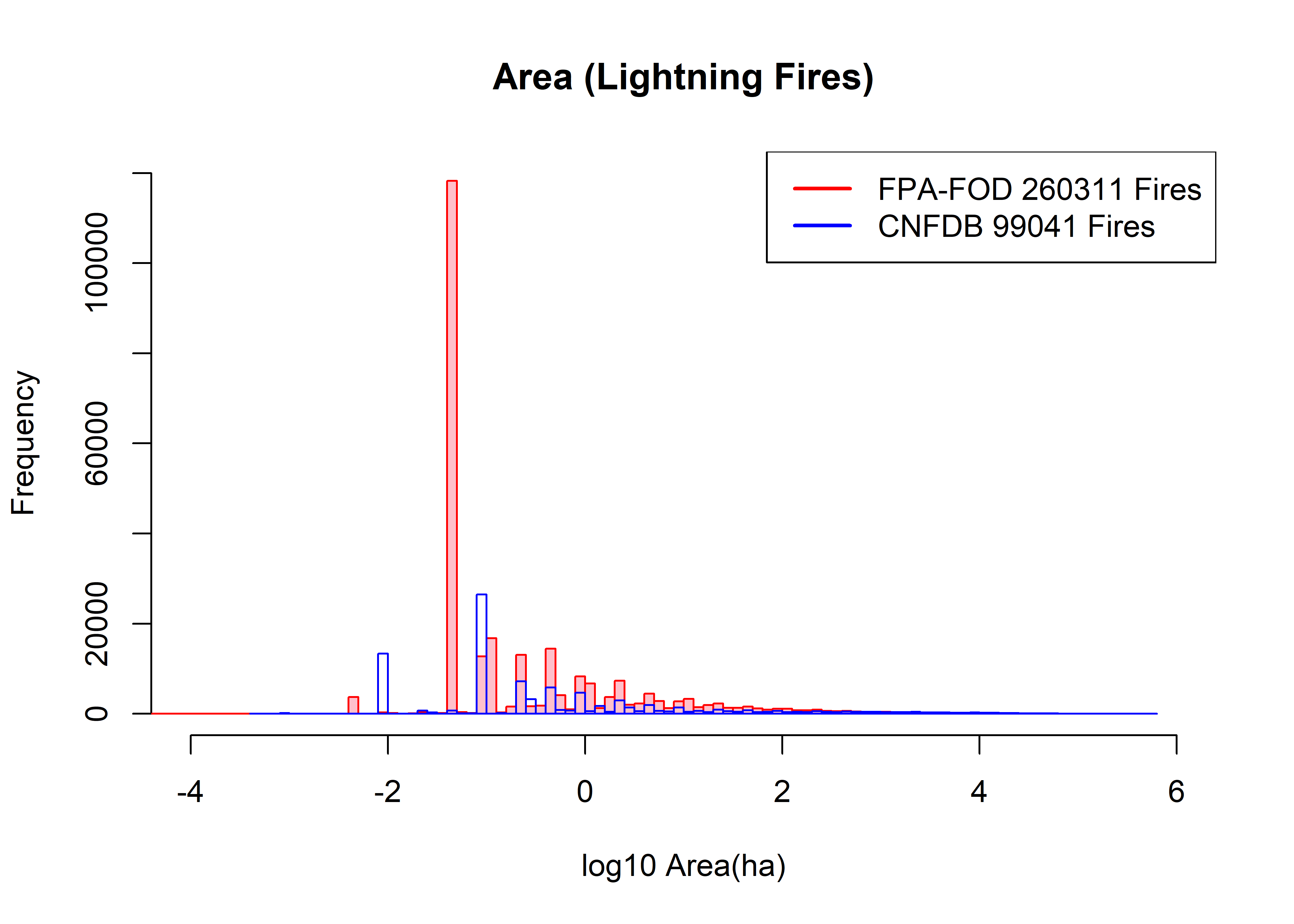
The main observation is that the histograms are quite “lumpy”, and don’t really smooth out until the size of fires reaches between 10 and 100 ha. The individual “spikes” in number of fires smaller than, say, 1 ha, are related to recording precision (e.g. 0.2, 0.4, etc. ha) or the acre-to-hectare conversion. For example, the large spike in US fires at 10^-1.3928 (113292) corresponds to fires coded as 0.1 acres (= 0.04069 ha), while the two spikes at 10^-2 (12755 fires) and 10^-1 (35126 fires) correspond to fires coded as 0.01 and 0.1 ha, respectively. Thus a lot of the detail at the small end of the size range in both data sets is probably artifactual.
Slightly wider bins don’t fix anything:
hist(log10(fpafod.lt$area_ha), xlim=c(-4,6), ylim=c(0,120000), breaks=50,
  col="pink", border="red", main="Area (Lightning Fires)", xlab="log10 Area")
hist(log10(cnfdb.lt$area_ha), xlim=c(-4,6), ylim=c(0,120000), breaks=50,
  col=NULL, border="blue", add=TRUE)
legend("topright", legend=c(paste("FPA-FOD",as.integer(fpafod.nfires0),"Fires"),
  paste("CNFDB",as.integer(cnfdb.nfires0),"Fires")), lwd=2, col=c("red","blue"))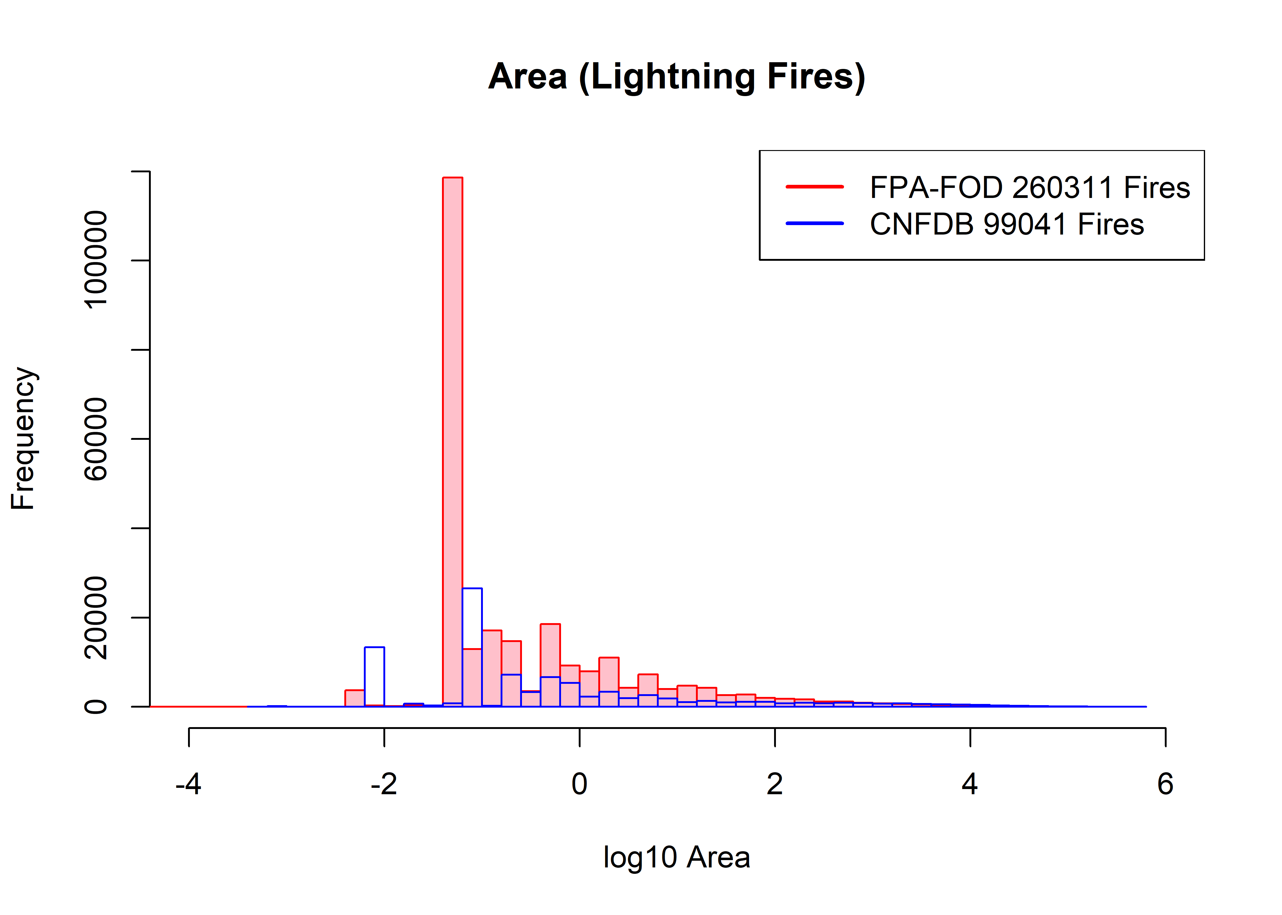
… and narrow bins seem even more noisier, and prone to effects of recording and transformation:
hist(log10(fpafod.lt$area_ha), xlim=c(-4,6), ylim=c(0,120000), breaks=200,
  col="pink", border="red", main="Area (Lightning Fires)", xlab="log10 Area")
hist(log10(cnfdb.lt$area_ha), xlim=c(-4,6), ylim=c(0,120000), breaks=200,
  col=NULL, border="blue", add=TRUE)
legend("topright", legend=c(paste("FPA-FOD",as.integer(fpafod.nfires0),"Fires"),
  paste("CNFDB",as.integer(cnfdb.nfires0),"Fires")), lwd=2, col=c("red","blue"))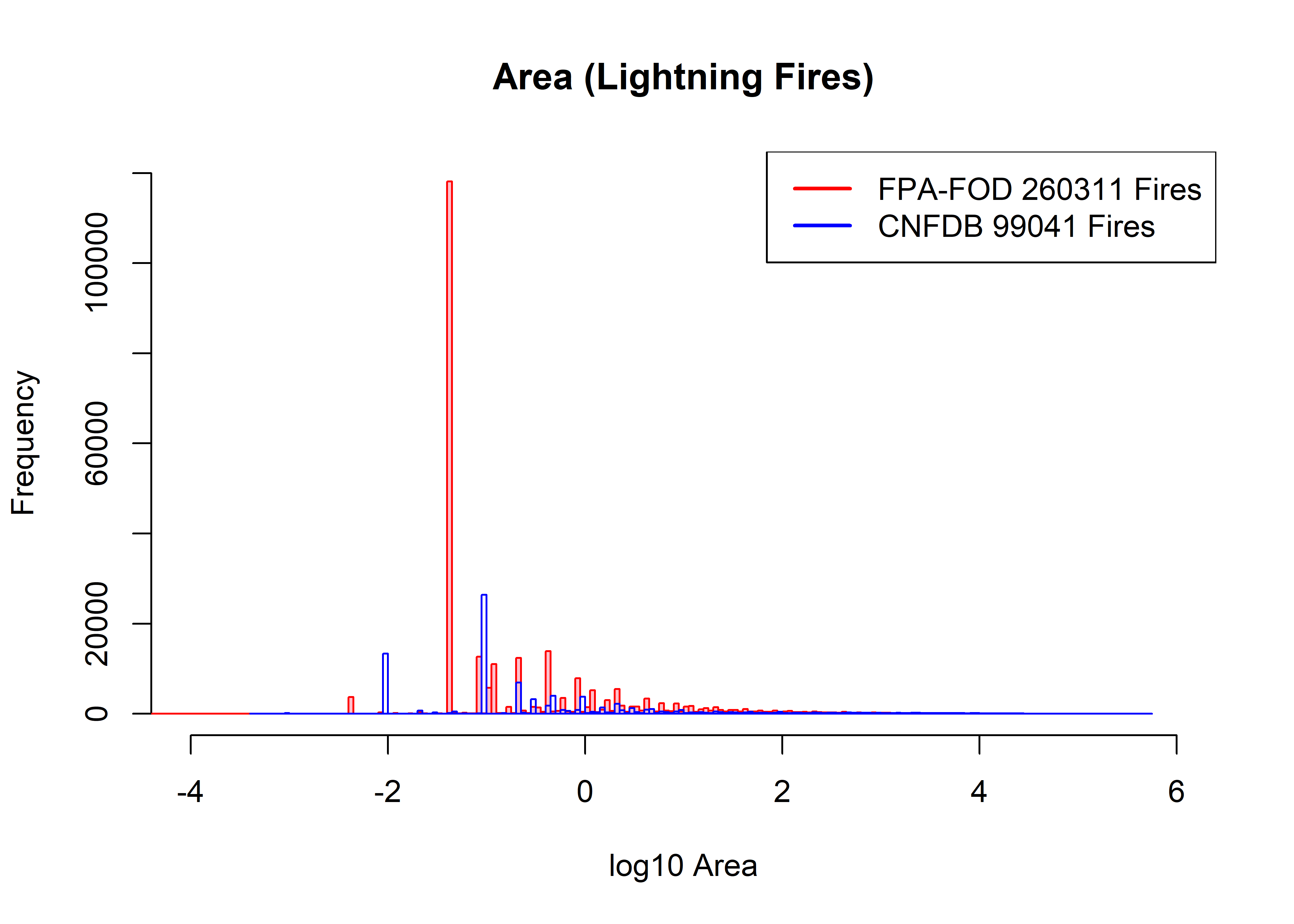
3.2 Area-Frequency Plots
So, at first glance, the distributions of the two data sets differ a lot, particularly at the low end. The question then becomes the role of the small fires, and where this is headed to is the question of whether, if the small fires are “censored” or removed, how comparable are the distributions of the large fires, and in particular, comparable enough to feel good about mergin the data sets. Ultimately we’re going to rely on how well the distribution of fires above some threshold can be represented by one or the other of the two extreme-value distributions (Pareto or tapered Pareto) the fire data gravitates toward. If the data “fit” one or the other (but the same) distributions that would argue that the underlying generating mechanisms in the two data sets are basically consistent with one another.
What follows is a bunch of frequency-area plots that illustrate the broad differences between the distributions (either number or size of fires) in the two data sets.
fpafod.nifires0 <- length(fpafod.lt$area_ha); cnfdb.nfires0 <- length(cnfdb.lt$area_ha)
plot(log10(fpafod.lt$area_ha), (seq(1,fpafod.nfires)), type="l", lwd=2, col="red",
  xlim=c(-4,6), xlab="log10(Area (ha))", ylab="Cumulative Total Number of Lightning Fires",
  main="Cumulative Total Number of Lighting Fires")
points(log10(cnfdb.lt$area_ha), (seq(1,cnfdb.nfires0)),
  cex=0.5, pch=16, type="l", lwd=2, col="blue")
legend("topleft", legend=c(paste("FPA-FOD",as.integer(fpafod.nfires)),
  paste("CNFDB",as.integer(cnfdb.nfires0))), lwd=2, col=c("red","blue"))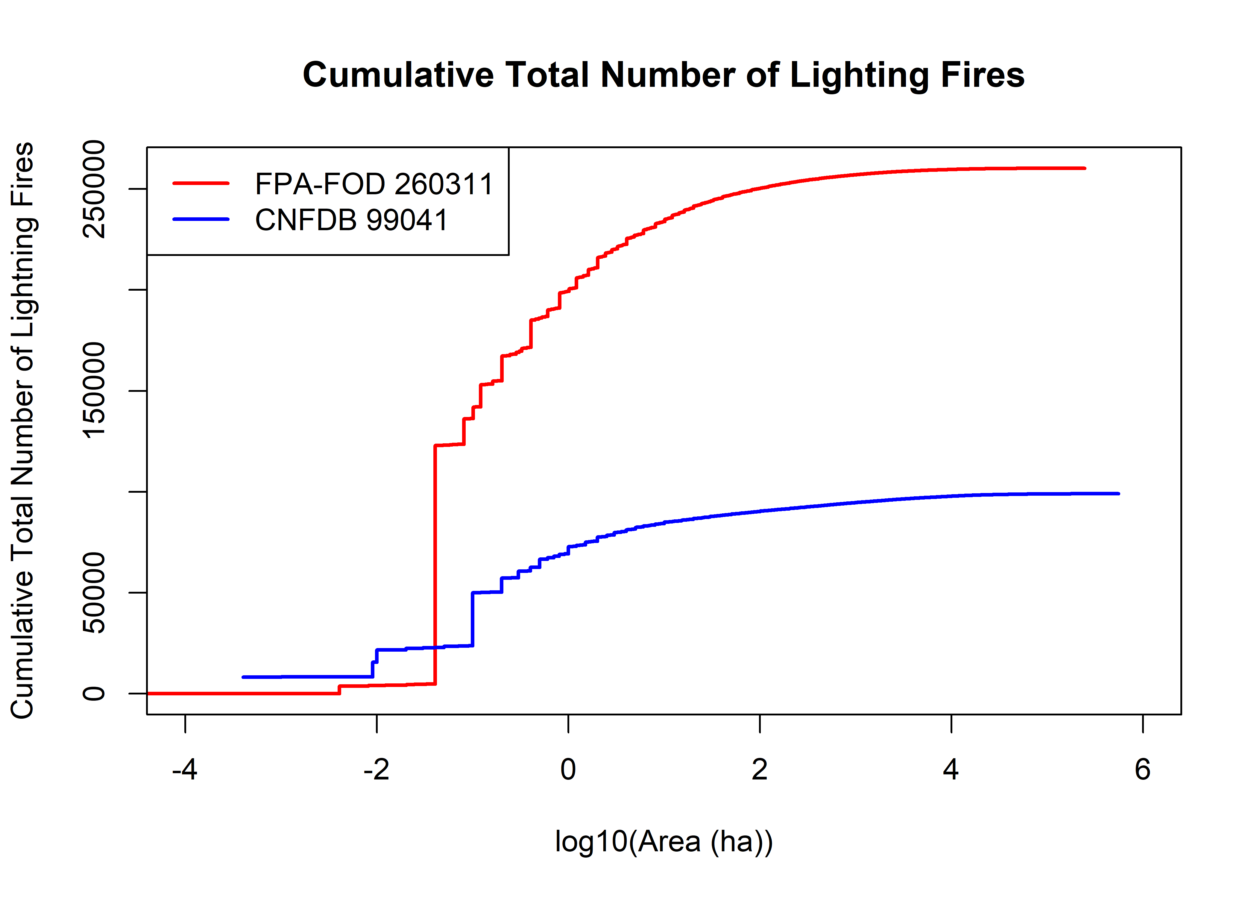
The above plot shows the cumulative number of fires as a function of fire size (on a logarthmic scale–there no really meaningful way to plot these data on a linear area scale). Just eyeballing this, it looks like in both data sets, roughly half of the fires are those with areas less than 10^-1 (0.1 ha). There over twice as many fires in the U.S> data set than in the Candadian data set, but the shapes of the curves are broadly similar.
plot(log10(fpafod.lt$area_ha), (seq(1,fpafod.nfires)/fpafod.nfires), type="l", lwd=2, col="red",
  xlim=c(-4,6), xlab="log10(Area (ha))", ylab="Cumulative Proportion",
  main="Cumulative Proportion of Total Number of Lighting Fires")
cnfdb.nfires0 <- length(cnfdb.lt$area_ha)
points(log10(cnfdb.lt$area_ha), (seq(1,cnfdb.nfires0)/cnfdb.nfires0),
  cex=0.5, pch=16, type="l", lwd=2, col="blue")
legend("topleft", legend=c(paste("FPA-FOD",as.integer(fpafod.nfires)),
  paste("CNFDB",as.integer(cnfdb.nfires0))), lwd=2, col=c("red","blue"))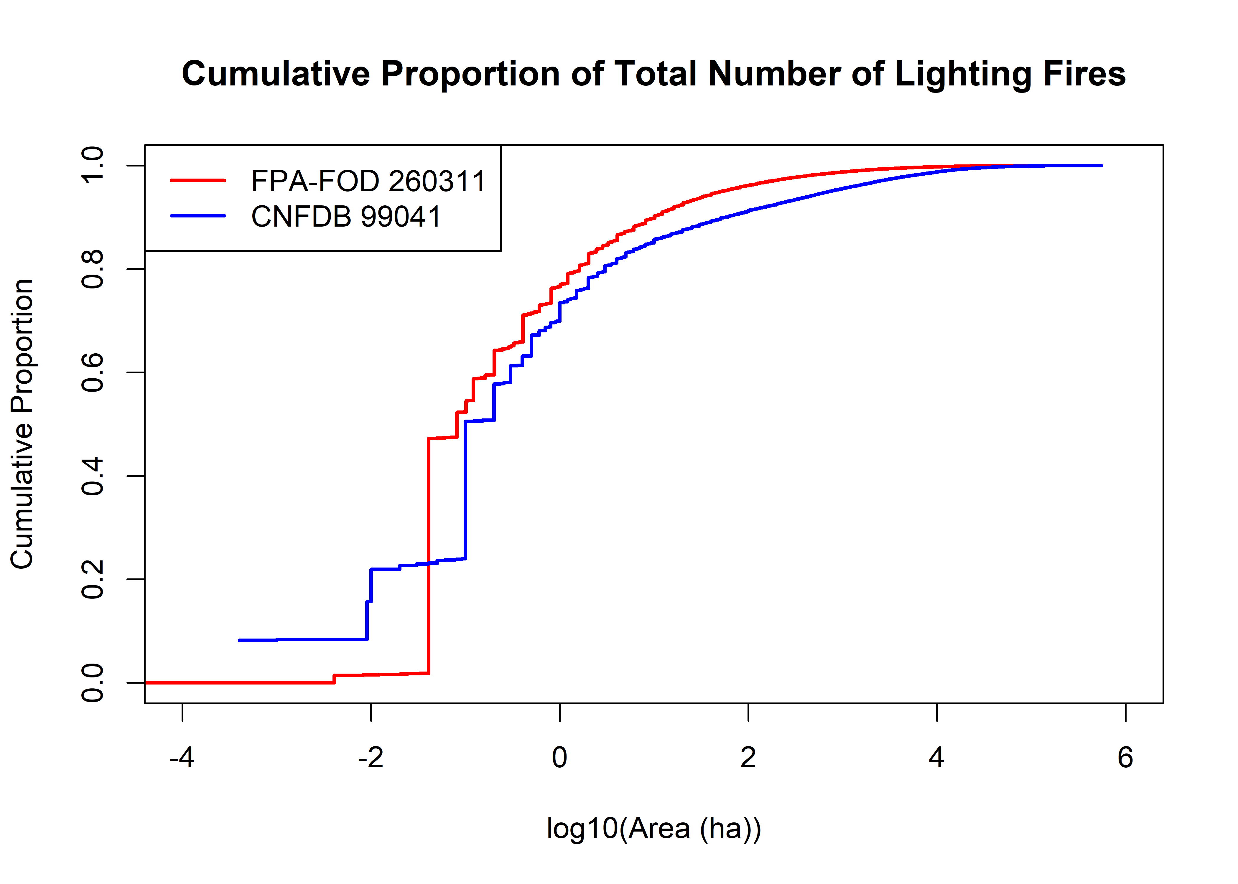
The plots above show the cumulative proportion of the total number of fires in each data set as a function of area, and makes it easier to see the implication of the first plot–roughly half of the fires in each data set are smaller than 0.1 ha, and half are bigger. That size of fire is relatively small in the general scheme of things, but they are quantatively important in terms of overall ignitions. Consequently it would not be good idea to simply just ignore them. However, importance in frequency is not necessarily importance in area.
fpafod.cumsum <- cumsum(fpafod.lt$area_ha); cnfdb.cumsum <- cumsum(cnfdb.lt$area_ha)
plot(log10(fpafod.lt$area_ha), fpafod.cumsum, main="Cumulative Area Burned (Lightning)", ylim=c(0,8e+7),
  cex=0.5, pch=16, type="l", col="red", lwd=2, xlim=c(-4,6), xlab="log10(AREA(ha))", ylab="Cumulative Area(ha)")
points(log10(cnfdb.lt$area_ha), cnfdb.cumsum,
  cex=0.5, pch=16, type="l", lwd=2, col="blue")
legend("topleft", legend=c(paste("FPA-FOD",as.integer(max(fpafod.cumsum)),"ha"),
  paste("CNFDB",as.integer(max(cnfdb.cumsum)),"ha")), lwd=2, col=c("red","blue"))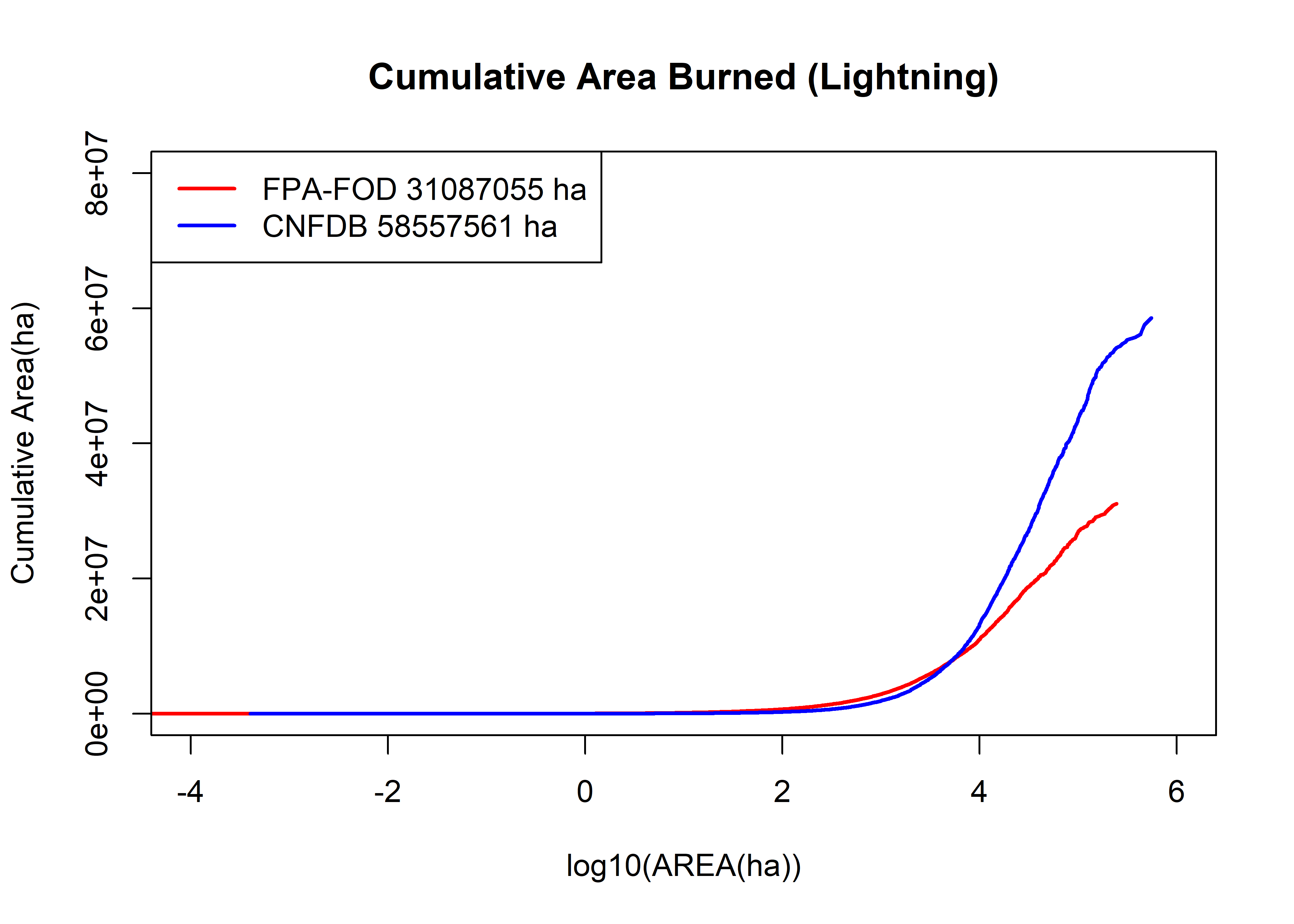
The above plot shows the cumulative area burned as a function of area. The first order observation is that the Canadian fires, while half as many in number as the U.S. fires, ultimately burn twice as much area. The two curves cross at around 3000 ha; above that area, Canadian fires dominate
fpafod.cumsum <- cumsum(fpafod.lt$area_ha); cnfdb.cumsum <- cumsum(cnfdb.lt$area_ha)
plot(log10(fpafod.lt$area_ha), (fpafod.cumsum/max(fpafod.cumsum)),
  main="Cumulative Proportion Total Area Burned (LIghtning)",
  cex=0.5, pch=16, type="l", col="red", lwd=2, xlim=c(-4,6),
  xlab="log10(AREA)", ylab="Cumulative Proportion")
points(log10(cnfdb.lt$area_ha), (cnfdb.cumsum/max(cnfdb.cumsum)),
  cex=0.5, pch=16, type="l", lwd=2, col="blue")
legend("topleft", legend=c(paste("FPA-FOD",as.integer(max(fpafod.cumsum)),"ha"),
  paste("CNFDB",as.integer(max(cnfdb.cumsum)),"ha")), lwd=2, col=c("red","blue"))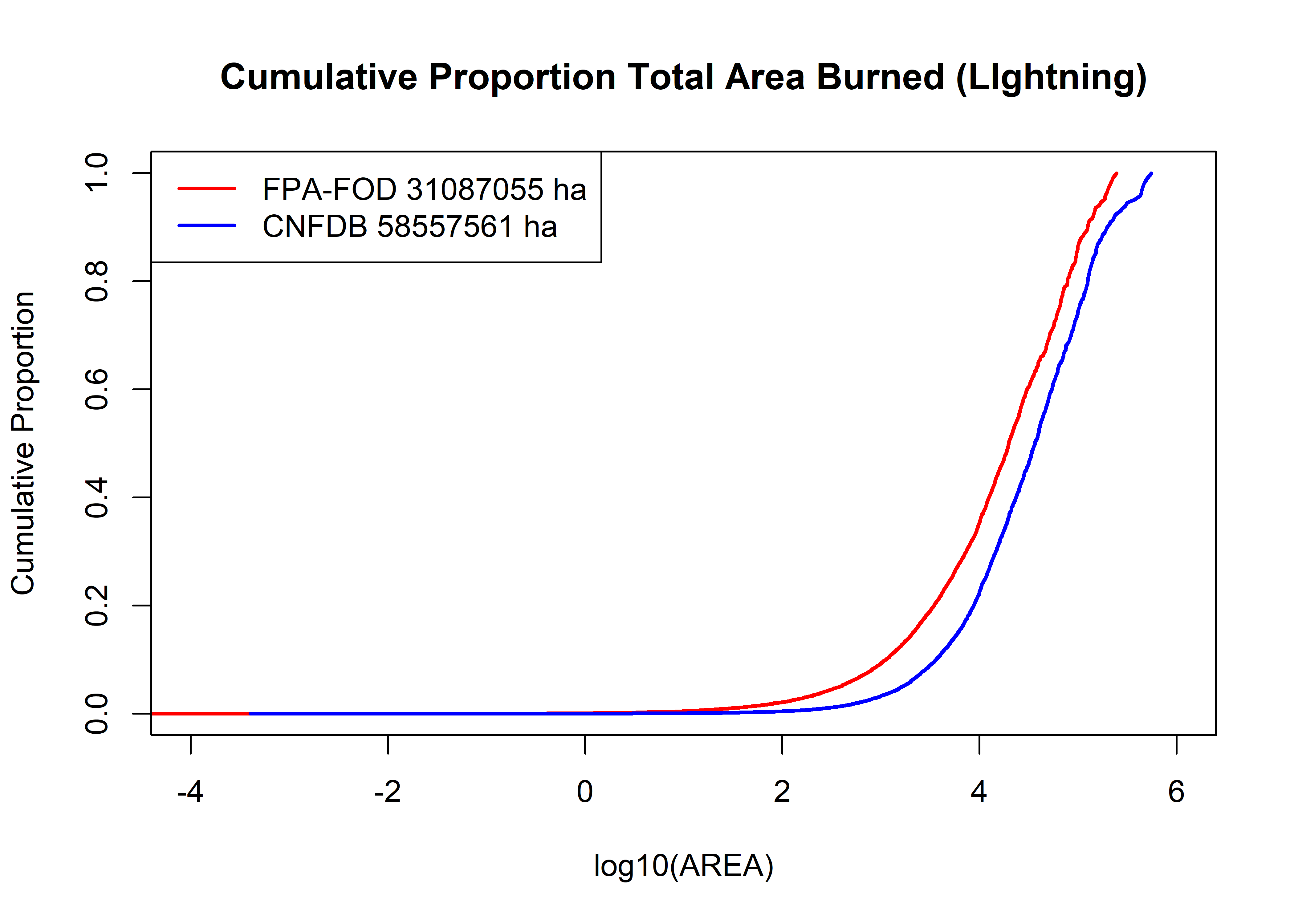
fpafod.cumsum <- cumsum(fpafod.lt$area_ha); cnfdb.cumsum <- cumsum(cnfdb.lt$area_ha)
plot(log10(fpafod.lt$area_ha), log10(fpafod.cumsum),
  main="Log10 Cumulative Area Burned (Lightning)", ylim=c(0,8e+7),
  cex=0.5, pch=16, type="l", col="red", lwd=2, xlim=c(-4,6), xlab="log10(AREA(ha))", ylab="Cumulative Area(ha)")
points(log10(cnfdb.lt$area_ha), cnfdb.cumsum,
  cex=0.5, pch=16, type="l", lwd=2, col="blue")
legend("topleft", legend=c(paste("FPA-FOD",as.integer(max(fpafod.cumsum)),"ha"),
  paste("CNFDB",as.integer(max(cnfdb.cumsum)),"ha")), lwd=2, col=c("red","blue"))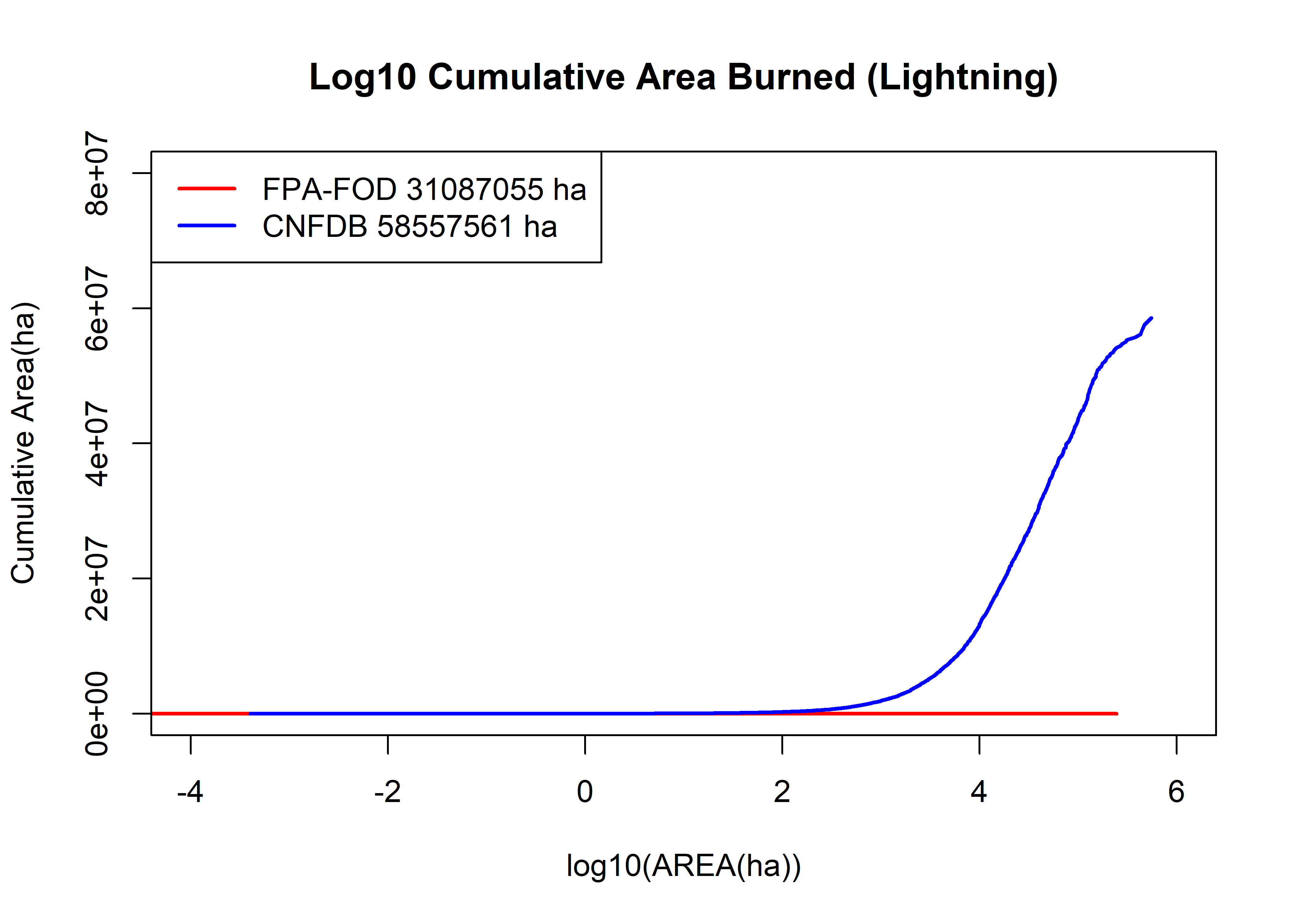
The greater frequency of large fires in the Canadian data set is evident in the above plot, which shows the proportion of the total area burned in each data set as a function of area. Above 10 ha, the shapes of the curves are roughtly similar, with the intermediate (10-1000 ha) large fires increasing more rapidly than in the Canadian data set.
Lastly, here are two “survivor curve” plots. The ordinate here is simply the rank of each fire (with 1 being the largest fire) divided by the total number of fires, which is thus the ratio of the number of fires greater in size than a particular area to the total number of fires. The curve gets it’s name from survival analysis, where it shows the number of individual that survive beyond time t divided by the total number of individuals, and it figures in fitting Pareto and tapered Pareto distributions. In an ideal world, where the beautiful physics of self-organizing complexity/fractality emerges as a fundimental law of everything, this should be a straight line.
Save the current workspace
outworkspace="all.lt.RData"
save.image(file=outworkspace)
4 More distribution plots and data binning
The next set of diagnostic plots require binning the data, and also “clipping”/“thresholding”/“truncating” the data, which will also come up later in fitting the Pareto and tapered Pareto distributions. The following code does this for the U.S. data.
First, define the bins and area threshold:
area.thresh <- -5.0
binbeg <- -4; binend <- 6; bw <- 0.2
breaks <- seq(binbeg, binend, by=bw); mid <- seq(binbeg+bw/2, binend-bw/2, by=bw)
head(breaks); tail(breaks)
## [1] -4.0 -3.8 -3.6 -3.4 -3.2 -3.0## [1] 5.0 5.2 5.4 5.6 5.8 6.0head(mid); tail(mid)## [1] -3.9 -3.7 -3.5 -3.3 -3.1 -2.9## [1] 4.9 5.1 5.3 5.5 5.7 5.94.1 US data, subsample and binning
# get data with areas > area.thres
farea.all <- fpafod.lt$area_ha
fname <- "FPA-FOD Lightning"
farea <- farea.all[farea.all > area.thresh]
farea.max <- max(farea); farea.min <- min(farea); fnfires <- length(farea)
farea.min; farea.max; fnfires; log10(farea.min); log10(farea.max)
## [1] 4.04686e-05## [1] 245622.1## [1] 260311## [1] -4.392882## [1] 5.390268# rank and survival curve values for clipped data
farea.index <-order(farea, na.last=FALSE)
head(farea[farea.index]);tail(farea[farea.index])## [1] 0.0000404686 0.0000404686 0.0000809372 0.0001857509 0.0004046860 0.0004046860## [1] 195576.7 202320.7 209254.2 217570.1 225895.0 245622.1farea <- farea[farea.index]
head(farea); tail(farea)## [1] 0.0000404686 0.0000404686 0.0000809372 0.0001857509 0.0004046860 0.0004046860## [1] 195576.7 202320.7 209254.2 217570.1 225895.0 245622.1farea.rank <- seq(fnfires, 1)
head(cbind(farea, farea.rank)); tail(cbind(farea, farea.rank))## farea farea.rank
## [1,] 0.0000404686 260311
## [2,] 0.0000404686 260310
## [3,] 0.0000809372 260309
## [4,] 0.0001857509 260308
## [5,] 0.0004046860 260307
## [6,] 0.0004046860 260306## farea farea.rank
## [260306,] 195576.7 6
## [260307,] 202320.7 5
## [260308,] 209254.2 4
## [260309,] 217570.1 3
## [260310,] 225895.0 2
## [260311,] 245622.1 1farea.surv <- (farea.rank)/fnfires
head(cbind(farea, farea.rank, farea.surv)); tail(cbind(farea, farea.rank, farea.surv))## farea farea.rank farea.surv
## [1,] 0.0000404686 260311 1.0000000
## [2,] 0.0000404686 260310 0.9999962
## [3,] 0.0000809372 260309 0.9999923
## [4,] 0.0001857509 260308 0.9999885
## [5,] 0.0004046860 260307 0.9999846
## [6,] 0.0004046860 260306 0.9999808## farea farea.rank farea.surv
## [260306,] 195576.7 6 2.304935e-05
## [260307,] 202320.7 5 1.920779e-05
## [260308,] 209254.2 4 1.536624e-05
## [260309,] 217570.1 3 1.152468e-05
## [260310,] 225895.0 2 7.683118e-06
## [260311,] 245622.1 1 3.841559e-06# bin the clipped data
#farea.hist <- hist(log10(farea), xlim=c(-4,6), breaks=100, plot=TRUE)
bin <- cut(log10(farea), breaks)
head(bin); tail(bin)## [1] <NA> <NA> <NA> (-3.8,-3.6] (-3.4,-3.2] (-3.4,-3.2]
## 50 Levels: (-4,-3.8] (-3.8,-3.6] (-3.6,-3.4] (-3.4,-3.2] (-3.2,-3] (-3,-2.8] (-2.8,-2.6] ... (5.8,6]## [1] (5.2,5.4] (5.2,5.4] (5.2,5.4] (5.2,5.4] (5.2,5.4] (5.2,5.4]
## 50 Levels: (-4,-3.8] (-3.8,-3.6] (-3.6,-3.4] (-3.4,-3.2] (-3.2,-3] (-3,-2.8] (-2.8,-2.6] ... (5.8,6]# binned variable values
fcount <- as.numeric(table(bin)); fcount## [1] 0 1 0 9 1 0 0 2 3728 274 168 429 181 118610 12917
## [16] 17077 14684 3482 18548 9261 7982 11015 4269 7242 3982 4757 4267 2647 2766 1986
## [31] 1828 1672 1190 1193 889 791 665 484 393 288 239 159 100 58 46
## [46] 18 10 0 0 0farea.ave <- as.numeric(tapply(farea, bin, mean)); farea.ave## [1] NA 1.857509e-04 NA 4.046860e-04 8.093720e-04 NA NA 3.237488e-03
## [9] 4.047837e-03 8.087251e-03 1.212854e-02 2.026260e-02 3.221837e-02 4.052798e-02 8.094972e-02 1.149207e-01
## [17] 2.001187e-01 3.138507e-01 4.493601e-01 8.067383e-01 1.209422e+00 1.974038e+00 3.140919e+00 4.891962e+00
## [25] 7.994302e+00 1.209535e+01 1.974774e+01 3.166950e+01 4.909544e+01 7.934079e+01 1.243812e+02 1.999103e+02
## [33] 3.138534e+02 4.965951e+02 7.998702e+02 1.254651e+03 2.003264e+03 3.158587e+03 4.987674e+03 8.044610e+03
## [41] 1.249274e+04 1.982989e+04 3.087900e+04 5.116925e+04 7.919328e+04 1.232216e+05 2.004002e+05 NA
## [49] NA NAfbin <- na.omit(data.frame(cbind(mid, 10^mid, farea.ave, fcount, farea.ave*fcount)))
names(fbin) <- c("logArea","Area.ha","aveSize","fireNum","CharFireSize")
fbin$surv <- (fnfires-cumsum(fbin$fireNum)+1)/fnfires
min.fsurv <- min(fbin$surv); max.fsurv <- max(fbin$surv)
max.fsurv; min.fsurv## [1] 1## [1] 1.536624e-05inv.rel.rank <- seq(0,1, by=1/(length(fbin$surv)-1))
fbin$surv <- (fbin$surv-min.fsurv)/(max.fsurv-min.fsurv) + inv.rel.rank*min.fsurv; fbin$fsurv## NULLhead(fbin); tail(fbin)## logArea Area.ha aveSize fireNum CharFireSize surv
## 2 -3.7 0.0001995262 0.0001857509 1 1.857509e-04 1.0000000
## 4 -3.3 0.0005011872 0.0004046860 9 3.642174e-03 0.9999658
## 5 -3.1 0.0007943282 0.0008093720 1 8.093720e-04 0.9999623
## 8 -2.5 0.0031622777 0.0032374880 2 6.474976e-03 0.9999550
## 9 -2.3 0.0050118723 0.0040478370 3728 1.509034e+01 0.9856338
## 10 -2.1 0.0079432823 0.0080872509 274 2.215907e+00 0.9845816## logArea Area.ha aveSize fireNum CharFireSize surv
## 42 4.3 19952.62 19829.89 159 3152953 9.047922e-04
## 43 4.5 31622.78 30879.00 100 3087900 5.209963e-04
## 44 4.7 50118.72 51169.25 58 2967817 2.985484e-04
## 45 4.9 79432.82 79193.28 46 3642891 1.221998e-04
## 46 5.1 125892.54 123221.62 18 2217989 5.341655e-05
## 47 5.3 199526.23 200400.16 10 2004002 1.536624e-054.2 Canadian data, subsample and binning
# get data with areas > area.threshold
carea.all <- cnfdb.lt$area_ha[cnfdb.lt$area_ha > 0]
cname <- "CNFDB Lightning" #
carea <- carea.all[carea.all > area.thresh]
carea.max <- max(carea); carea.min <- min(carea); cnfires <- length(carea)
carea.min; carea.max; cnfires; log10(carea.min); log10(carea.max)
## [1] 4e-04## [1] 553680## [1] 90887## [1] -3.39794## [1] 5.743259# rank and survival curve values for clipped data
carea.index <-order(carea, na.last=FALSE)
head(carea[carea.index]);tail(carea[carea.index])## [1] 4e-04 1e-03 1e-03 1e-03 1e-03 1e-03## [1] 428100.0 438000.0 453144.0 466420.3 501689.1 553680.0carea <- carea[carea.index]
head(carea); tail(carea)## [1] 4e-04 1e-03 1e-03 1e-03 1e-03 1e-03## [1] 428100.0 438000.0 453144.0 466420.3 501689.1 553680.0carea.rank <- seq(cnfires, 1)
head(cbind(carea, carea.rank)); tail(cbind(carea, carea.rank))## carea carea.rank
## [1,] 4e-04 90887
## [2,] 1e-03 90886
## [3,] 1e-03 90885
## [4,] 1e-03 90884
## [5,] 1e-03 90883
## [6,] 1e-03 90882## carea carea.rank
## [90882,] 428100.0 6
## [90883,] 438000.0 5
## [90884,] 453144.0 4
## [90885,] 466420.3 3
## [90886,] 501689.1 2
## [90887,] 553680.0 1carea.surv <- (carea.rank)/cnfires
head(cbind(carea, carea.rank, carea.surv)); tail(cbind(carea, carea.rank, carea.surv))## carea carea.rank carea.surv
## [1,] 4e-04 90887 1.000000
## [2,] 1e-03 90886 0.999989
## [3,] 1e-03 90885 0.999978
## [4,] 1e-03 90884 0.999967
## [5,] 1e-03 90883 0.999956
## [6,] 1e-03 90882 0.999945## carea carea.rank carea.surv
## [90882,] 428100.0 6 6.601604e-05
## [90883,] 438000.0 5 5.501337e-05
## [90884,] 453144.0 4 4.401069e-05
## [90885,] 466420.3 3 3.300802e-05
## [90886,] 501689.1 2 2.200535e-05
## [90887,] 553680.0 1 1.100267e-05# bin the clipped data
#carea.hist <- hist(log10(carea), xlim=c(-4,6), breaks=100, plot=TRUE)
bin <- cut(log10(carea), breaks)
head(bin); tail(bin)## [1] (-3.4,-3.2] (-3.2,-3] (-3.2,-3] (-3.2,-3] (-3.2,-3] (-3.2,-3]
## 50 Levels: (-4,-3.8] (-3.8,-3.6] (-3.6,-3.4] (-3.4,-3.2] (-3.2,-3] (-3,-2.8] (-2.8,-2.6] ... (5.8,6]## [1] (5.6,5.8] (5.6,5.8] (5.6,5.8] (5.6,5.8] (5.6,5.8] (5.6,5.8]
## 50 Levels: (-4,-3.8] (-3.8,-3.6] (-3.6,-3.4] (-3.4,-3.2] (-3.2,-3] (-3,-2.8] (-2.8,-2.6] ... (5.8,6]# binned variable values
ccount <- as.numeric(table(bin)); ccount## [1] 0 0 0 1 137 0 7 10 25 13380 28 713 291 769 26546 212 7200
## [18] 3290 6653 5378 2303 3398 1934 2628 1886 1042 1287 969 1143 1085 771 893 804 906
## [35] 836 709 748 618 556 522 420 288 197 143 76 57 17 5 6 0carea.ave <- as.numeric(tapply(carea, bin, mean)); carea.ave## [1] NA NA NA 4.000000e-04 1.000000e-03 NA 2.000000e-03 3.000000e-03
## [9] 5.160000e-03 9.459043e-03 1.367857e-02 2.004067e-02 3.010309e-02 4.877503e-02 9.984103e-02 1.405519e-01
## [17] 2.014361e-01 3.005465e-01 4.853192e-01 9.236928e-01 1.393619e+00 2.075559e+00 3.128392e+00 4.850731e+00
## [25] 8.600337e+00 1.323903e+01 2.069925e+01 3.173713e+01 4.963518e+01 8.388658e+01 1.293604e+02 2.044208e+02
## [33] 3.185556e+02 5.028512e+02 8.076753e+02 1.285331e+03 2.022932e+03 3.168852e+03 4.989494e+03 8.069331e+03
## [41] 1.255250e+04 1.977460e+04 3.145060e+04 4.941208e+04 8.048821e+04 1.260371e+05 1.959858e+05 3.077275e+05
## [49] 4.735056e+05 NAcbin <- na.omit(data.frame(cbind(mid, 10^mid, carea.ave, ccount, carea.ave*ccount)))
names(cbin) <- c("logArea","Area.ha","aveSize","fireNum","CharFireSize")
cbin$surv <- (cnfires-cumsum(cbin$fireNum)+1)/cnfires
min.csurv <- min(cbin$surv); max.csurv <- max(cbin$surv)
max.csurv; min.csurv## [1] 1## [1] 1.100267e-05inv.rel.rank <- seq(0,1, by=1/(length(cbin$surv)-1))
cbin$surv <- (cbin$surv-min.csurv)/(max.csurv-min.csurv) + inv.rel.rank*min.csurv; cbin$csurv## NULLhead(cbin); tail(cbin)## logArea Area.ha aveSize fireNum CharFireSize surv
## 4 -3.3 0.0005011872 0.000400000 1 0.0004 1.0000000
## 5 -3.1 0.0007943282 0.001000000 137 0.1370 0.9984929
## 7 -2.7 0.0019952623 0.002000000 7 0.0140 0.9984161
## 8 -2.5 0.0031622777 0.003000000 10 0.0300 0.9983063
## 9 -2.3 0.0050118723 0.005160000 25 0.1290 0.9980315
## 10 -2.1 0.0079432823 0.009459043 13380 126.5620 0.8508144## logArea Area.ha aveSize fireNum CharFireSize surv
## 44 4.7 50118.72 49412.08 143 7065928 1.781202e-03
## 45 4.9 79432.82 80488.21 76 6117104 9.452400e-04
## 46 5.1 125892.54 126037.11 57 7184115 3.183307e-04
## 47 5.3 199526.23 195985.77 17 3331758 1.315333e-04
## 48 5.5 316227.77 307727.46 5 1538637 7.676938e-05
## 49 5.7 501187.23 473505.57 6 2841033 1.100267e-054.3 Plots of binned data
Impact of binning on the distributions (and the shape of the survival-function plot in particular).
plot(log10(farea), log10(farea.surv), type="l", pch=16, xlim=c(-4,6), ylim=c(-5,0),
  cex=0.5, lwd=3, ylab="log10(S(x))", xlab="log10(Area(ha))", col="pink", main="Impact of Binning")
points(fbin$logArea, log10(fbin$surv), type="o", pch=16, cex=0.8, lwd=2, col="red")
points(log10(carea), log10(carea.surv), type="l", pch=16, cex=0.5, lwd=3, col="lightblue")
points(cbin$logArea, log10(cbin$surv), type="o", pch=16, cex=0.8, lwd=2, col="blue")
legend("bottomleft", legend=c("FPA-FOD","FPA-FOD Binned","CNFDB","CNFDB Binned"), lwd=3,
  col=c("pink","red","lightblue","blue"))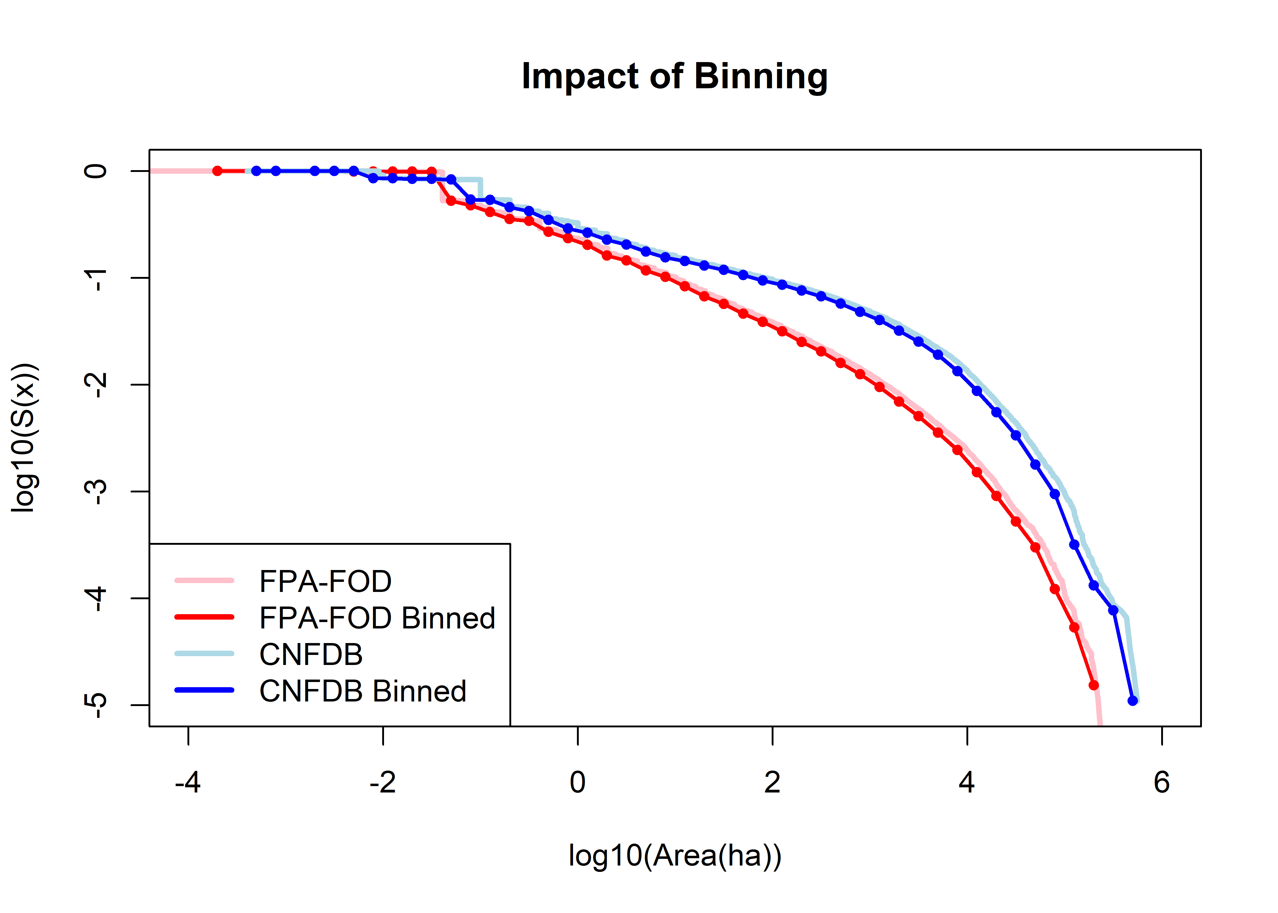
No impact on the overall shape of the distributions.
Below is the “characteristic fires-size” plot of Lehsten et al.
plot(cbin$logArea, cbin$CharFireSize, xlim=c(-4,6), type="h", col="blue", lwd=3,
  main="Characteristic Fire Sizes")
points(fbin$logArea+.05, fbin$CharFireSize, xlim=c(-4,6), type="h", col="red", lwd=3)
legend("topleft", legend=c("FPA-FOD","CNFDB"), lwd=3, col=c("red","blue"))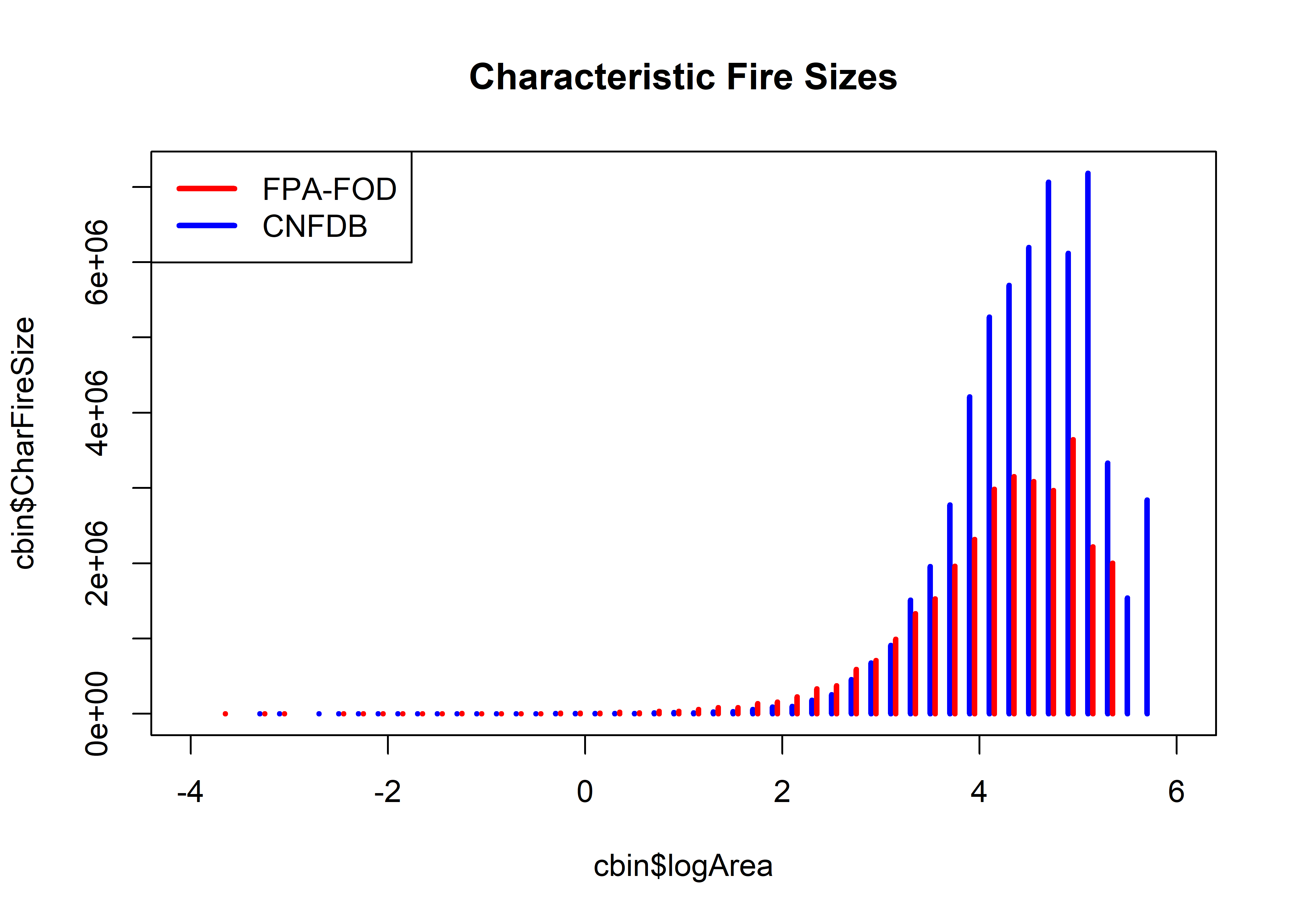
The overall appearance of this plot shound be like the normal distribution (if the data follow a power-law type of generating process). Both distributions are clearly truncated at the high end, and don’t look too symetric in the middle range of fire sizes.
The next plot is the Sachs et al. frequency-area plot, with least-squres “power-law” fits.
plot(fbin$logArea, log10(fbin$fireNum/fbin$Area.ha), xlim=c(-4,6), xlab="log10(Area(ha))",
  ylab="log10(fireNum/Area.ha)", ylim=c(-6,8), pch=16, col="red", main=paste(fname,"Frequency-Area Relationship"))
f.lm.power <- lm(log10(fbin$fireNum/fbin$Area.ha) ~ fbin$logArea)
f.lm.power2 <- lm(log10(fbin$fireNum/fbin$Area.ha)[log10(fbin$Area.ha) >=0] ~ fbin$logArea[log10(fbin$Area.ha) >=0])
abline(f.lm.power, col="pink", lwd=2); abline(f.lm.power2, col="red", lwd=2)
points(cbin$logArea, log10(cbin$fireNum/cbin$Area.ha), pch=16, col="blue")
c.lm.power <- lm(log10(cbin$fireNum/cbin$Area.ha) ~ cbin$logArea)
c.lm.power2 <- lm(log10(cbin$fireNum/cbin$Area.ha)[log10(cbin$Area.ha) >=0] ~ cbin$logArea[log10(cbin$Area.ha) >=0])
abline(c.lm.power, col="lightblue", lwd=2); abline(c.lm.power2, col="blue", lwd=2)
legend("bottomleft", legend=c(paste("FPA-FOD slope=",round(f.lm.power$coefficients[2], digits=4)),
  paste("FPA-FOD > 1.0 ha, slope=",round(f.lm.power2$coefficients[2], digits=4)),
  paste("CNFDB slope=",round(c.lm.power$coefficients[2], digits=4)),
  paste("CNFDB > 1.0 ha, slope=",round(c.lm.power2$coefficients[2], digits=4))),
  lwd=2, col=c("pink","red","lightblue","blue"))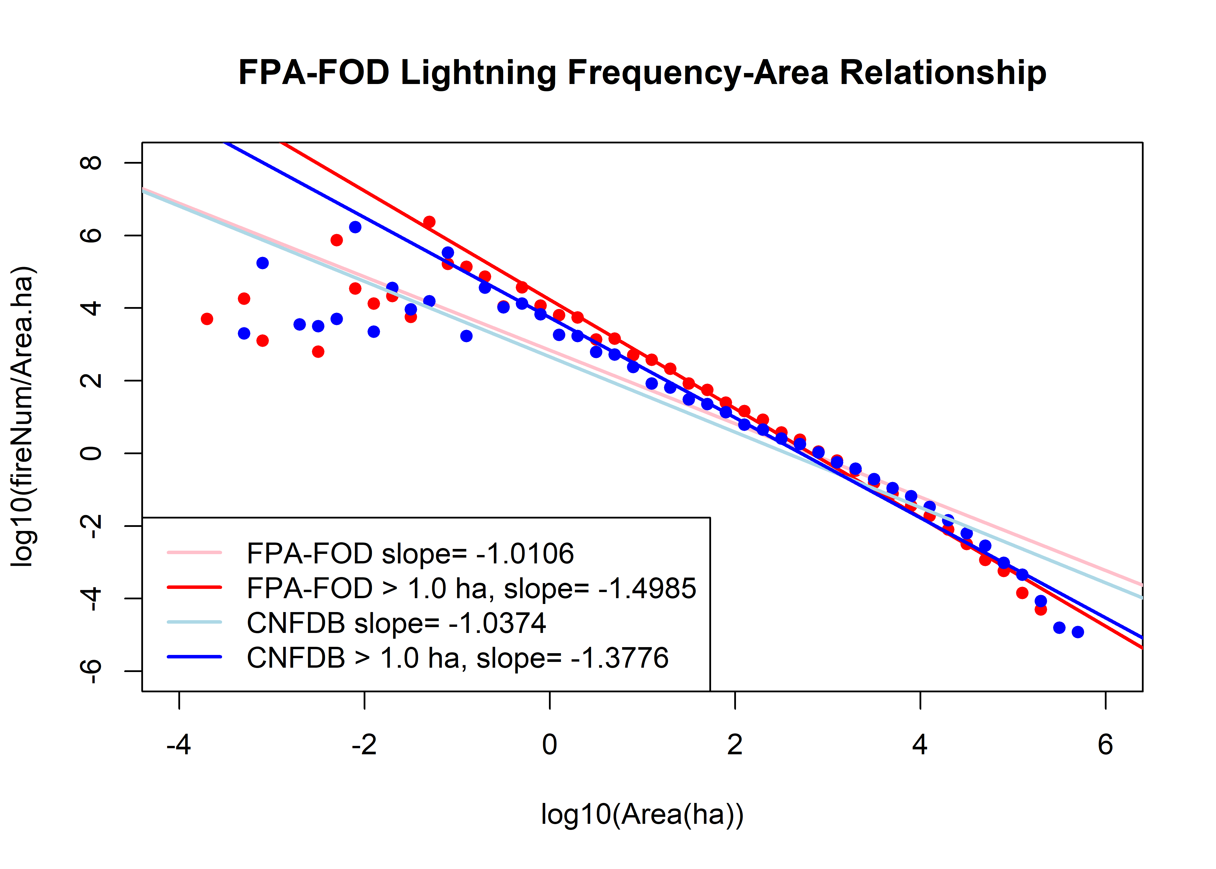
Lot’s going on here. First, the fits to the whole data sets (light curves), fit terribly. The fits to just the data greater than 1.0 ha look superficially better, but underestimate the “frequency density” for fires greater than 100 ha, and overestimate the largest fires. This is diagnostic of a poor fit by a power-law relationship.
5 Pareto and tapered-Pareto distributions
The following analyses are patterned after those in Schoenberg, et al. (2003, Environmetrics 14:585-592), in which a number of different distributions were fit to the Los Angeles County fire data. There the analysis involved fitting several distributions to the fire data, including the Pareto distribution, which follows directly from the idea that fires have a power-law distribution, and the tapered-Pareto distribution which also has a general physical explantion, but turns out to fit the data much better for large fires. The distributions can be fit by maximizing the log-likelihood of the distibutions, which didn’t seem to work well, or by (nonlinear) least squares applied to the relationship between the “survivor function” and the pdf of each distribution.
Fitting the distributions is highly dependent on good starting values, and so the first step was interatively trying a range of values for the parameters, a, the lower truncation point, which can be regarded as known (from consideration of the way in which the data were generated–a could be considered the size threshold at which the records become complete), beta, the shape parameter, and theta which can be regarded as an upper area threshold above which the frequency of large fires rapidly decreases.
The following code fits the Pareto and tapered-Pareto distributions (and plots the results. First, the U.S. data, assuming that a is equal to 1.0 ha.
Load the lightning-only data from the previous steps.
5.1 US Data
5.1.1 Rank and survival-curve data
Note that this overwrites previous data…
area.thresh = 1.0 # ha
fpafod.lt.area <- fpafod.lt$area_ha[fpafod.lt$area_ha > area.thresh]
fpafod.lt.name <- "Merged U.S. Lightning Data"
fpafod.lt.area.max <- max(fpafod.lt.area); fpafod.lt.area.min <- min(fpafod.lt.area)
fpafod.lt.nfires <- length(fpafod.lt.area)
cbind(fpafod.lt.area.max, fpafod.lt.area.min, fpafod.lt.nfires)
## fpafod.lt.area.max fpafod.lt.area.min fpafod.lt.nfires
## [1,] 245622.1 1.003621 60936fpafod.lt.area.index <- order(fpafod.lt.area, na.last=FALSE)
head(fpafod.lt.area.index); tail(fpafod.lt.area.index)## [1] 1 2 3 4 5 6## [1] 60931 60932 60933 60934 60935 60936Sort the area data, and get survival-curve ordinates.
fpafod.lt.area.sort <- fpafod.lt.area[fpafod.lt.area.index]
fpafod.lt.area.rank <- seq(fpafod.lt.nfires, 1)
fpafod.lt.area.surv <- fpafod.lt.area.rank/fpafod.lt.nfires
head(cbind(fpafod.lt.area.sort, fpafod.lt.area.rank, fpafod.lt.area.surv))
## fpafod.lt.area.sort fpafod.lt.area.rank fpafod.lt.area.surv
## [1,] 1.003621 60936 1.0000000
## [2,] 1.003621 60935 0.9999836
## [3,] 1.003621 60934 0.9999672
## [4,] 1.007668 60933 0.9999508
## [5,] 1.011715 60932 0.9999344
## [6,] 1.011715 60931 0.9999179tail(cbind(fpafod.lt.area.sort, fpafod.lt.area.rank, fpafod.lt.area.surv))## fpafod.lt.area.sort fpafod.lt.area.rank fpafod.lt.area.surv
## [60931,] 195576.7 6 9.846396e-05
## [60932,] 202320.7 5 8.205330e-05
## [60933,] 209254.2 4 6.564264e-05
## [60934,] 217570.1 3 4.923198e-05
## [60935,] 225895.0 2 3.282132e-05
## [60936,] 245622.1 1 1.641066e-055.1.2 Initial fits
Plot the observed survivor curve (in red) and that estimated by the Pareto and tapered-Pareto distributions, using guesses of the parameter values.
# Initital values of parameters
a0 <- area.thresh
beta0 <- 0.40
theta0 <-  30000.0

plot(log10(fpafod.lt.area.sort), log10(fpafod.lt.area.surv),
  type="l", pch=16, cex=0.5, lwd=2, col="red", xlim=c(-1,6), ylim=c(-6,0),
  xlab="log10(Area)", ylab="log10(S(x)", main=paste(fpafod.lt.name,"Fires >",as.character(a0),"ha"))
abline(0, -0.5, col="gray", lwd=2)

fpafod.lt.fx.pareto <- 1.0 - (a0/fpafod.lt.area.sort)^beta0
head(fpafod.lt.fx.pareto); tail(fpafod.lt.fx.pareto)
## [1] 0.001444851 0.001444851 0.001444851 0.003050892 0.004647929 0.004647929## [1] 0.9923533 0.9924563 0.9925573 0.9926724 0.9927817 0.9930194points(log10(fpafod.lt.area.sort), log10(1.0 - fpafod.lt.fx.pareto), col="blue", type="l", lwd=2)
fpafod.lt.fx.tappareto <- 1.0 - ((a0/fpafod.lt.area.sort)^beta0)*exp((a0-fpafod.lt.area.sort)/theta0)
head(fpafod.lt.fx.tappareto); tail(fpafod.lt.fx.tappareto)## [1] 0.001444971 0.001444971 0.001444971 0.003051147 0.004648318 0.004648318## [1] 0.9999887 0.9999911 0.9999930 0.9999948 0.9999961 0.9999981points(log10(fpafod.lt.area.sort), log10(1.0 - fpafod.lt.fx.tappareto), type="l", pch=16, cex=0.5, col="purple", lwd=2)
legend("bottomleft", title="by hand", legend=c("Observed","Pareto","Tapered Parto",
"slope = -0.5"), lwd=2, col=c("red","blue","purple","gray"))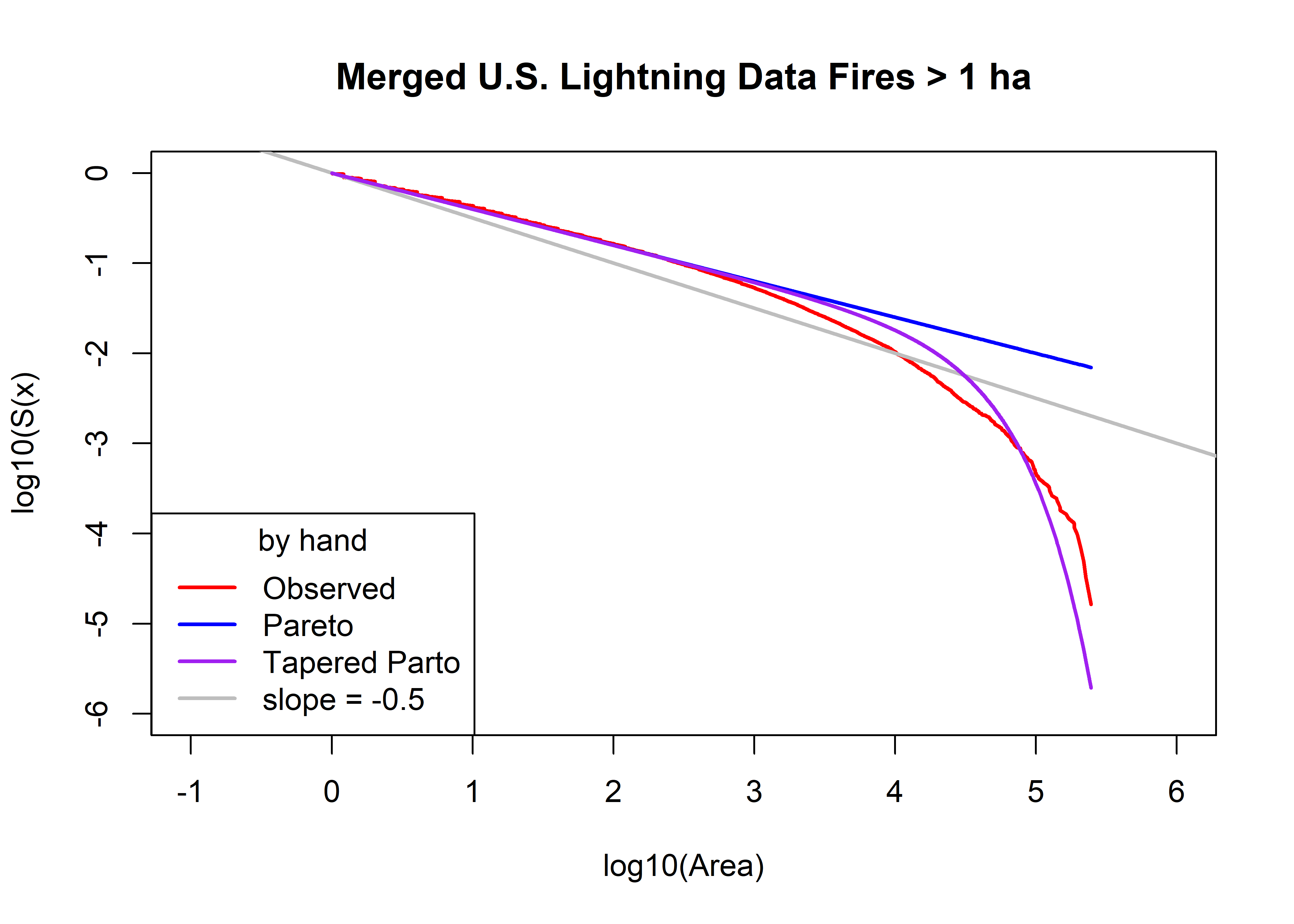
5.1.3 Optimization
# optim() estimation Pareto
SSE.Pareto <- function(p, data, surv){
  y <- log10(surv)
  yhat <- log10((p[2]/data)^p[1])
  x <- sum((y-yhat)^2.0)
  return(x)
}
p0 <- c(beta0, a0); p0
## [1] 0.4 1.0#data=farea; surv=farea.surv
fit.Pareto <- optim(p0, SSE.Pareto, data=fpafod.lt.area.sort, surv=fpafod.lt.area.surv )
beta1 <- fit.Pareto$par[1]; a1 <- fit.Pareto$par[2]; sse1 <- fit.Pareto$value
beta1; a1; sse1## [1] 0.4519132## [1] 1.305437## [1] 315.9868# optim() estimation tapered Pareto
SSE.tapPareto <- function(p, data, surv){
y <- log10(surv)
yhat <- log10(((p[3]/data)^p[1])*exp((p[3]-data)/p[2]))
x <- sum((y-yhat)^2.0)
return(x)
}
p2 <- c(beta0, theta0, a0); p2## [1] 4e-01 3e+04 1e+00fit.tapPareto1 <- optim(p2, SSE.tapPareto, data=fpafod.lt.area.sort, surv=fpafod.lt.area.surv)
beta2 <- fit.tapPareto1$par[1]; theta2 <- fit.tapPareto1$par[2]
a2 <- fit.tapPareto1$par[3]; sse2 <- fit.tapPareto1$value
beta2; theta2; a2; sse2## [1] 0.4274505## [1] 31143.76## [1] 1.194998## [1] 85.04488# optim() estimation tapered Pareto -- a fixed
SSE.tapPareto2 <- function(p, data, surv, a){
y <- log10(surv)
yhat <- log10( ((a/data)^p[1])*exp((a-data)/p[2]) )
x <- sum((y-yhat)^2.0)
return(x)
}
p3 <- c(beta0, theta0); p3; a <- a0## [1] 4e-01 3e+04fit.tapPareto2 <- optim(p3, SSE.tapPareto2, data=fpafod.lt.area.sort, a=a, surv=fpafod.lt.area.surv)
beta3 <- fit.tapPareto2$par[1]; theta3 <- fit.tapPareto2$par[2]
a3 <- a0; sse3 <- fit.tapPareto2$value
beta3; theta3; a3; sse3## [1] 0.4091267## [1] 29101.31## [1] 1## [1] 112.9372# compare observed and fitted
plot(log10(fpafod.lt.area.sort), log10(fpafod.lt.area.surv), type="n", ylim=c(-5,0), xlim=c(-1,6),
xlab="log10(Area)", ylab="log10(S(x)", main=paste(fpafod.lt.name,"Fires >",as.character(a0),"ha"))
abline(log10(fpafod.lt.area.min)/2, -0.5, col="gray", lwd=2)
fpafod.lt.fx.pareto <- 1.0 - (a1/fpafod.lt.area.sort)^beta1
head(fpafod.lt.fx.pareto); tail(fpafod.lt.fx.pareto)## [1] -0.1261653 -0.1261653 -0.1261653 -0.1241192 -0.1220849 -0.1220849## [1] 0.9954176 0.9954872 0.9955554 0.9956330 0.9957065 0.9958659points(log10(fpafod.lt.area.sort), log10(1.0 - fpafod.lt.fx.pareto), col="blue", type="l", lwd=2)
fpafod.lt.fx.tappareto <- 1.0 - ((a2/fpafod.lt.area.sort)^beta2)*exp((a2-fpafod.lt.area.sort)/theta2)
head(fpafod.lt.fx.tappareto); tail(fpafod.lt.fx.tappareto)## [1] -0.07746264 -0.07746264 -0.07746264 -0.07561072 -0.07376939 -0.07376939## [1] 0.9999889 0.9999912 0.9999931 0.9999948 0.9999961 0.9999980points(log10(fpafod.lt.area.sort), log10(1.0 - fpafod.lt.fx.tappareto), col="purple", type="l", lwd=2)
fpafod.lt.fx.tappareto <- 1.0 - ((a3/fpafod.lt.area.sort)^beta3)*exp((a3-fpafod.lt.area.sort)/theta3)
head(fpafod.lt.fx.tappareto); tail(fpafod.lt.fx.tappareto)## [1] 0.001477917 0.001477917 0.001477917 0.003120657 0.004754128 0.004754128## [1] 0.9999917 0.9999935 0.9999950 0.9999963 0.9999973 0.9999987points(log10(fpafod.lt.area.sort), log10(1.0 - fpafod.lt.fx.tappareto), col="pink", type="l", lwd=2)
points(log10(fpafod.lt.area.sort), log10(fpafod.lt.area.surv), pch=16, cex=0.5, col="red")
legend("bottomleft", title="optim() fit", legend=c("FPA-FOD","Pareto","Tapered Pareto",
"Tapered Pareto (a fixed)", "slope = -0.5"), lwd=2, col=c("red","blue","purple","pink","gray"))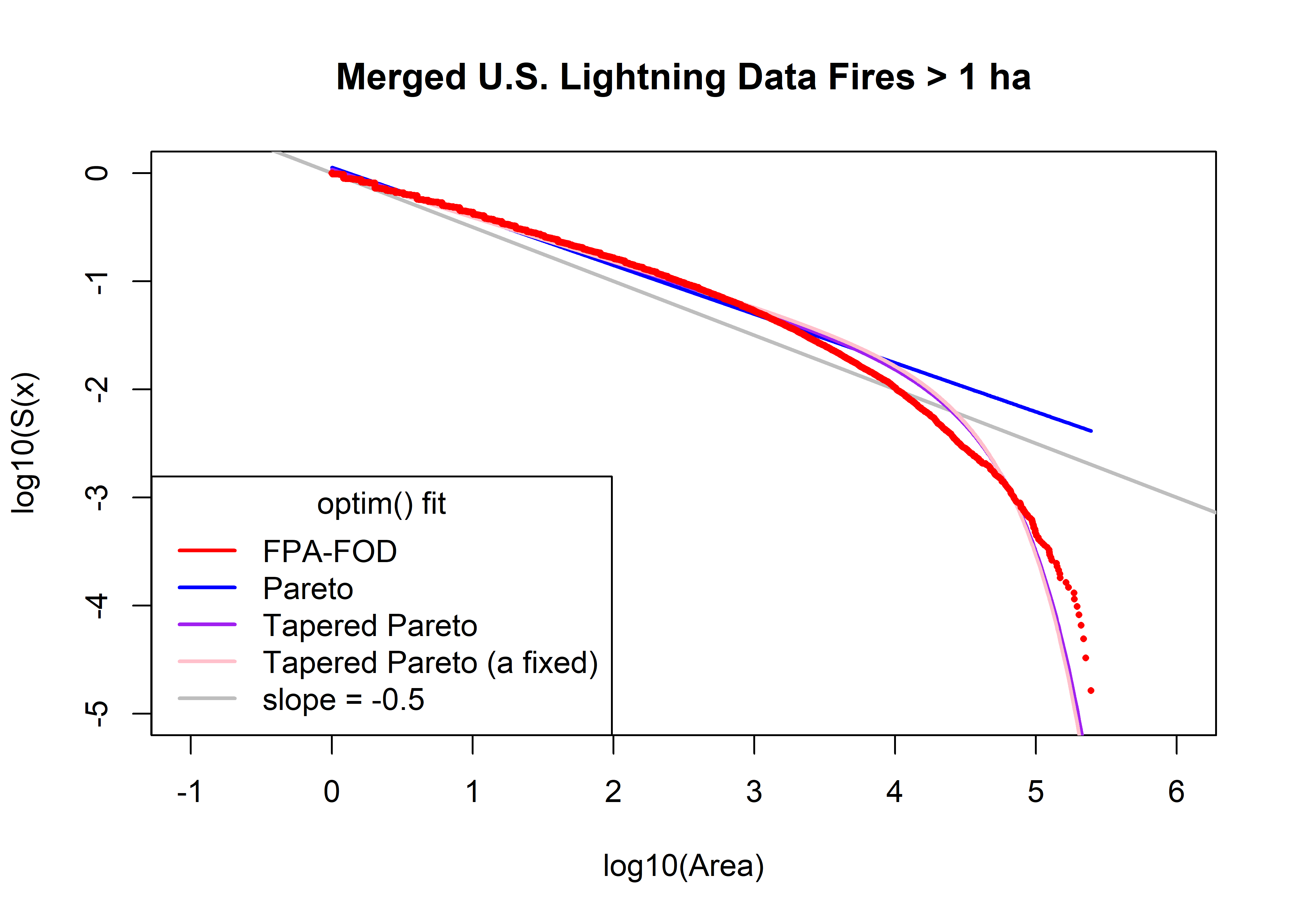
print(cbind(beta0, theta0, a0, beta1, a1, sse1, beta2, theta2, a2, sse2, beta3, theta3, a3, sse3))## beta0 theta0 a0 beta1 a1 sse1 beta2 theta2 a2 sse2 beta3 theta3 a3
## [1,] 0.4 30000 1 0.4519132 1.305437 315.9868 0.4274505 31143.76 1.194998 85.04488 0.4091267 29101.31 1
## sse3
## [1,] 112.9372us.beta0 <- beta0; us.theta0 <- theta0; us.a0 <- a0; us.beta1 <- beta1; us.a1 <- a1;
us.beta2 <- beta2; us.theta2 <- theta3; us.a2 <- a2;
us.beta3 <- beta3; us.theta3 <- theta3; us.a3 <- a35.1.4 QQ Plots
library(PtProcess)
fpafod.lt.area.prob <- ppoints(fpafod.lt.area.sort)
qp <- qpareto(fpafod.lt.area.prob, beta1, a1, lower.tail=TRUE, log.p=FALSE)
head(qp); tail(qp)
## [1] 1.305460 1.305508 1.305555 1.305603 1.305650 1.305698## [1] 1162807886 1812821817 3161342547 6656190698 20612744973 234377836430qtap <- qtappareto(fpafod.lt.area.prob, beta2, theta2, a2, lower.tail=TRUE, log.p=FALSE, tol=1e-8)
head(qtap); tail(qtap)## [1] 1.195021 1.195067 1.195112 1.195158 1.195204 1.195250## [1] 135136.0 140835.6 148001.8 157640.9 172361.5 204312.5head(cbind(log10(fpafod.lt.area.sort),qp,qtap,log10(qp),log10(qtap),fpafod.lt.area.prob))## qp qtap fpafod.lt.area.prob
## [1,] 0.001569861 1.305460 1.195021 0.1157637 0.07737540 8.205330e-06
## [2,] 0.001569861 1.305508 1.195067 0.1157795 0.07739208 2.461599e-05
## [3,] 0.001569861 1.305555 1.195112 0.1157953 0.07740875 4.102665e-05
## [4,] 0.003317527 1.305603 1.195158 0.1158110 0.07742542 5.743731e-05
## [5,] 0.005058189 1.305650 1.195204 0.1158268 0.07744209 7.384797e-05
## [6,] 0.005058189 1.305698 1.195250 0.1158426 0.07745877 9.025863e-05tail(cbind(log10(fpafod.lt.area.sort),qp,qtap,log10(qp),log10(qtap),fpafod.lt.area.prob))## qp qtap fpafod.lt.area.prob
## [60931,] 5.291317 1162807886 135136.0 9.065508 5.130771 0.9999097
## [60932,] 5.306040 1812821817 140835.6 9.258355 5.148713 0.9999262
## [60933,] 5.320674 3161342547 148001.8 9.499872 5.170267 0.9999426
## [60934,] 5.337599 6656190698 157640.9 9.823226 5.197669 0.9999590
## [60935,] 5.353907 20612744973 172361.5 10.314136 5.236440 0.9999754
## [60936,] 5.390268 234377836430 204312.5 11.369917 5.310295 0.9999918plot(log10(fpafod.lt.area.sort), log10(qtap), xlim=c(-1,6), ylim=c(-1,6), xlab="Observed log10(Area)", type="n",
ylab="log10(Theoretical Quantiles)", main=paste("QQPlot",fpafod.lt.name,"Fires >",as.character(a0),"ha"))
abline(0.0, 1.0, col="gray", lwd=2)
points(log10(fpafod.lt.area.sort),log10(qp), type="l", col="blue", lwd=2)
points(log10(fpafod.lt.area.sort),log10(qtap), type="l", col="purple", lwd=2)
legend("topleft", legend=c("Pareto","Tapered Pareto"), lwd=2, col=c("blue","purple"))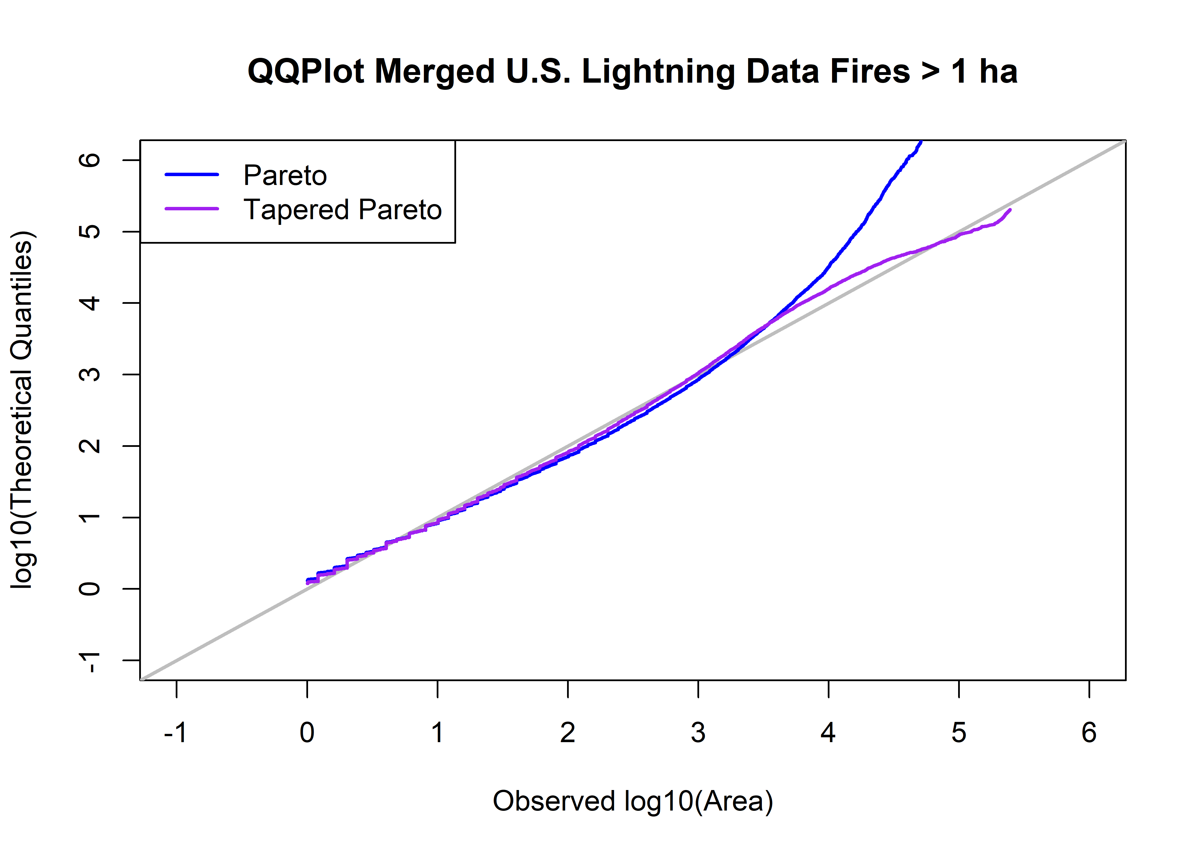
5.2 Canadian data
5.2.1 Rank and survival-curve data
Note that this overwrites previous data…
area.thresh = 1.0 # ha
cnfdb.lt.area <- cnfdb.lt$area_ha[cnfdb.lt$area_ha > area.thresh]
cnfdb.lt.name <- "Canada Lightning Data"
cnfdb.lt.area.max <- max(cnfdb.lt.area); cnfdb.lt.area.min <- min(cnfdb.lt.area)
cnfdb.lt.nfires <- length(cnfdb.lt.area)
cbind(cnfdb.lt.area.max, cnfdb.lt.area.min, cnfdb.lt.nfires)
## cnfdb.lt.area.max cnfdb.lt.area.min cnfdb.lt.nfires
## [1,] 553680 1.02 26247cnfdb.lt.area.index <- order(cnfdb.lt.area, na.last=FALSE)
head(cnfdb.lt.area.index); tail(cnfdb.lt.area.index)## [1] 1 2 3 4 5 6## [1] 26242 26243 26244 26245 26246 26247Sort the area data, and get survival-curve ordinates.
cnfdb.lt.area.sort <- cnfdb.lt.area[cnfdb.lt.area.index]
cnfdb.lt.area.rank <- seq(cnfdb.lt.nfires, 1)
cnfdb.lt.area.surv <- cnfdb.lt.area.rank/cnfdb.lt.nfires
head(cbind(cnfdb.lt.area.sort, cnfdb.lt.area.rank, cnfdb.lt.area.surv))
## cnfdb.lt.area.sort cnfdb.lt.area.rank cnfdb.lt.area.surv
## [1,] 1.02 26247 1.0000000
## [2,] 1.02 26246 0.9999619
## [3,] 1.04 26245 0.9999238
## [4,] 1.05 26244 0.9998857
## [5,] 1.05 26243 0.9998476
## [6,] 1.05 26242 0.9998095tail(cbind(cnfdb.lt.area.sort, cnfdb.lt.area.rank, cnfdb.lt.area.surv))## cnfdb.lt.area.sort cnfdb.lt.area.rank cnfdb.lt.area.surv
## [26242,] 428100.0 6 2.285976e-04
## [26243,] 438000.0 5 1.904980e-04
## [26244,] 453144.0 4 1.523984e-04
## [26245,] 466420.3 3 1.142988e-04
## [26246,] 501689.1 2 7.619918e-05
## [26247,] 553680.0 1 3.809959e-055.2.2 Initial fits
Plot the observed survivor curve (in red) and that estimated by the Pareto and tapered-Pareto distributions, using guesses of the parameter values.
# intital values of parameters
a0 <- area.thresh
beta0 <- 0.4
theta0 <-  30000.0

plot(log10(cnfdb.lt.area.sort), log10(cnfdb.lt.area.surv),
  type="l", pch=16, cex=0.5, lwd=2, col="red", xlim=c(-1,6), ylim=c(-6,0),
  xlab="log10(Area)", ylab="log10(S(x)", main=paste(cnfdb.lt.name,"Fires >",as.character(a0),"ha"))
abline(0, -0.5, col="gray", lwd=2)

cnfdb.lt.fx.pareto <- 1.0 - (a0/cnfdb.lt.area.sort)^beta0
head(cnfdb.lt.fx.pareto); tail(cnfdb.lt.fx.pareto)
## [1] 0.007889762 0.007889762 0.015565865 0.019326860 0.019326860 0.019326860## [1] 0.9944104 0.9944613 0.9945361 0.9945988 0.9947540 0.9949569points(log10(cnfdb.lt.area.sort), log10(1.0 - cnfdb.lt.fx.pareto), col="blue", type="l", lwd=2)
cnfdb.lt.fx.tappareto <- 1.0 - ((a0/cnfdb.lt.area.sort)^beta0)*exp((a0-cnfdb.lt.area.sort)/theta0)
head(cnfdb.lt.fx.tappareto); tail(cnfdb.lt.fx.tappareto)## [1] 0.007890423 0.007890423 0.015567178 0.019328495 0.019328495 0.019328495## [1] 1 1 1 1 1 1points(log10(cnfdb.lt.area.sort), log10(1.0 - cnfdb.lt.fx.tappareto), type="l", pch=16, cex=0.5, col="purple", lwd=2)
legend("bottomleft", title="by hand", legend=c("Observed","Pareto","Tapered Parto",
"slope = -0.5"), lwd=2, col=c("red","blue","purple","gray"))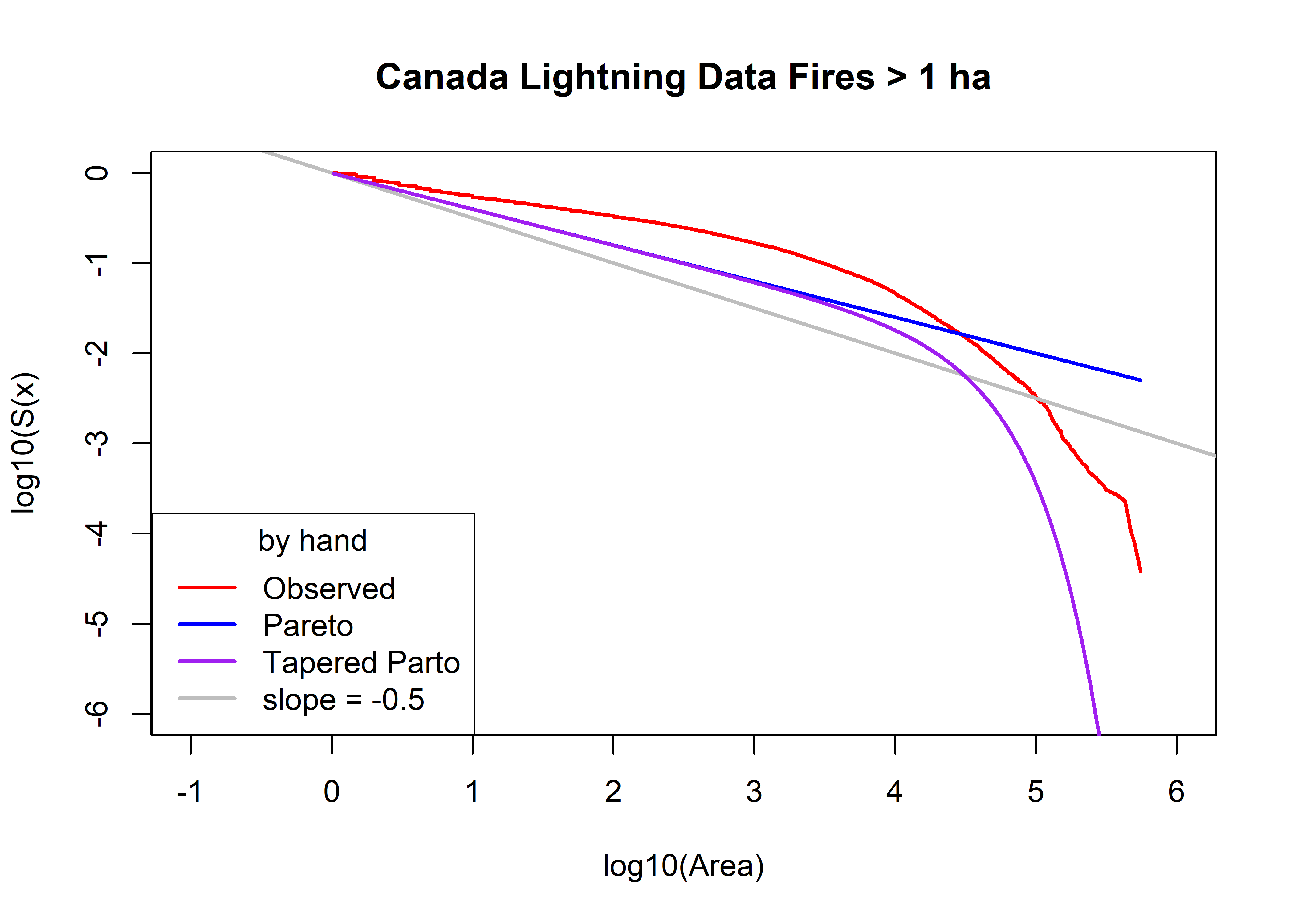
5.2.3 Optimization
# optim() estimation Pareto
SSE.Pareto <- function(p, data, surv){
  y <- log10(surv)
  yhat <- log10((p[2]/data)^p[1])
  x <- sum((y-yhat)^2.0)
  return(x)
}
p0 <- c(beta0, a0); p0
## [1] 0.4 1.0#data=farea; surv=farea.surv
fit.Pareto <- optim(p0, SSE.Pareto, data=cnfdb.lt.area.sort, surv=cnfdb.lt.area.surv )
beta1 <- fit.Pareto$par[1]; a1 <- fit.Pareto$par[2]; sse1 <- fit.Pareto$value
beta1; a1; sse1## [1] 0.3302408## [1] 1.771774## [1] 453.2954# optim() estimation tapered Pareto
SSE.tapPareto <- function(p, data, surv){
y <- log10(surv)
yhat <- log10(((p[3]/data)^p[1])*exp((p[3]-data)/p[2]))
x <- sum((y-yhat)^2.0)
return(x)
}
p2 <- c(beta0, theta0, a0); p2## [1] 4e-01 3e+04 1e+00fit.tapPareto1 <- optim(p2, SSE.tapPareto, data=cnfdb.lt.area.sort, surv=cnfdb.lt.area.surv)
beta2 <- fit.tapPareto1$par[1]; theta2 <- fit.tapPareto1$par[2]
a2 <- fit.tapPareto1$par[3]; sse2 <- fit.tapPareto1$value
beta2; theta2; a2; sse2## [1] 0.2922834## [1] 47551.18## [1] 1.404053## [1] 129.922# optim() estimation tapered Pareto -- a fixed
SSE.tapPareto2 <- function(p, data, surv, a){
y <- log10(surv)
yhat <- log10( ((a/data)^p[1])*exp((a-data)/p[2]) )
x <- sum((y-yhat)^2.0)
return(x)
}
p3 <- c(beta0, theta0); p3; a <- a0## [1] 4e-01 3e+04fit.tapPareto2 <- optim(p3, SSE.tapPareto2, data=cnfdb.lt.area.sort, a=a, surv=cnfdb.lt.area.surv)
beta3 <- fit.tapPareto2$par[1]; theta3 <- fit.tapPareto2$par[2]
a3 <- a0; sse3 <- fit.tapPareto2$value
beta3; theta3; a3; sse3## [1] 0.2743276## [1] 45259.99## [1] 1## [1] 148.0754# compare observed and fitted
plot(log10(cnfdb.lt.area.sort), log10(cnfdb.lt.area.surv), type="n", ylim=c(-5,0), xlim=c(-1,6),
xlab="log10(Area)", ylab="log10(S(x)", main=paste(cnfdb.lt.name,"Fires >",as.character(a0),"ha"))
abline(log10(cnfdb.lt.area.min)/2, -0.5, col="gray", lwd=2)
cnfdb.lt.fx.pareto <- 1.0 - (a1/cnfdb.lt.area.sort)^beta1
head(cnfdb.lt.fx.pareto); tail(cnfdb.lt.fx.pareto)## [1] -0.2000364 -0.2000364 -0.1923656 -0.1886034 -0.1886034 -0.1886034## [1] 0.9833172 0.9834427 0.9836275 0.9837829 0.9841686 0.9846759points(log10(cnfdb.lt.area.sort), log10(1.0 - cnfdb.lt.fx.pareto), col="blue", type="l", lwd=2)
cnfdb.lt.fx.tappareto <- 1.0 - ((a2/cnfdb.lt.area.sort)^beta2)*exp((a2-cnfdb.lt.area.sort)/theta2)
head(cnfdb.lt.fx.tappareto); tail(cnfdb.lt.fx.tappareto)## [1] -0.09791203 -0.09791203 -0.09169793 -0.08864849 -0.08864849 -0.08864849## [1] 0.9999969 0.9999975 0.9999982 0.9999987 0.9999994 0.9999998points(log10(cnfdb.lt.area.sort), log10(1.0 - cnfdb.lt.fx.tappareto), col="purple", type="l", lwd=2)
cnfdb.lt.fx.tappareto <- 1.0 - ((a3/cnfdb.lt.area.sort)^beta3)*exp((a3-cnfdb.lt.area.sort)/theta3)
head(cnfdb.lt.fx.tappareto); tail(cnfdb.lt.fx.tappareto)## [1] 0.005418117 0.005418117 0.010702523 0.013296404 0.013296404 0.013296404## [1] 0.9999978 0.9999982 0.9999987 0.9999991 0.9999996 0.9999999points(log10(cnfdb.lt.area.sort), log10(1.0 - cnfdb.lt.fx.tappareto), col="pink", type="l", lwd=2)
points(log10(cnfdb.lt.area.sort), log10(cnfdb.lt.area.surv), pch=16, cex=0.5, col="red")
legend("bottomleft", title="optim() fit", legend=c("FPA-FOD","Pareto","Tapered Pareto",
"Tapered Pareto (a fixed)", "slope = -0.5"), lwd=2, col=c("red","blue","purple","pink","gray"))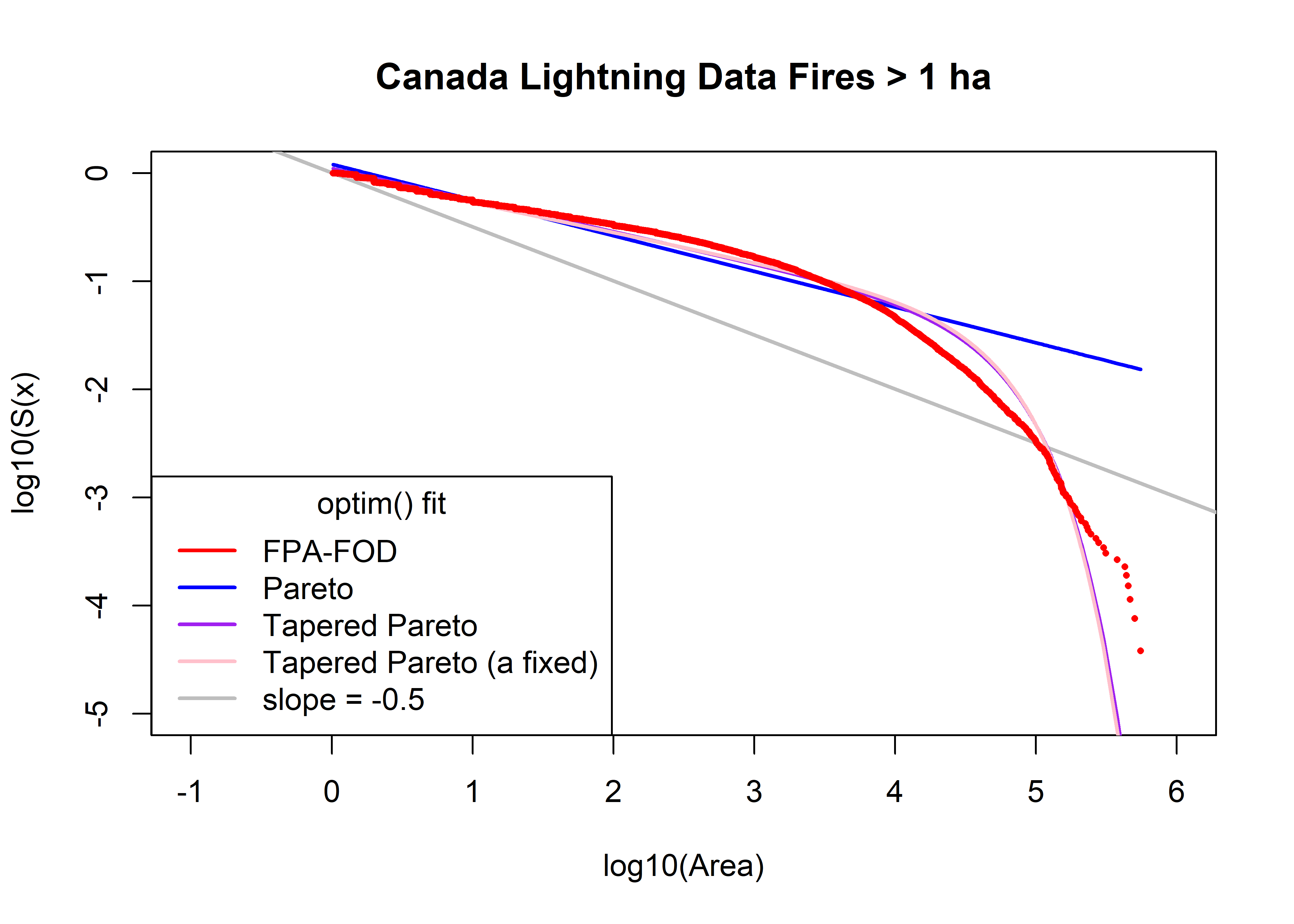
print(cbind(beta0, theta0, a0, beta1, a1, sse1, beta2, theta2, a2, sse2, beta3, theta3, a3, sse3))## beta0 theta0 a0 beta1 a1 sse1 beta2 theta2 a2 sse2 beta3 theta3 a3
## [1,] 0.4 30000 1 0.3302408 1.771774 453.2954 0.2922834 47551.18 1.404053 129.922 0.2743276 45259.99 1
## sse3
## [1,] 148.0754can.beta0 <- beta0; can.theta0 <- theta0; can.a0 <- a0; can.beta1 <- beta1; can.a1 <- a1;
can.beta2 <- beta2; can.theta2 <- theta3; can.a2 <- a2;
can.beta3 <- beta3; can.theta3 <- theta3; can.a3 <- a35.2.4 QQ Plots
library(PtProcess)
cnfdb.lt.area.prob <- ppoints(cnfdb.lt.area.sort)
qp <- qpareto(cnfdb.lt.area.prob, beta1, a1, lower.tail=TRUE, log.p=FALSE)
head(qp); tail(qp)
## [1] 1.771876 1.772080 1.772285 1.772489 1.772694 1.772898## [1] 2.442909e+11 4.485452e+11 9.600766e+11 2.659471e+12 1.249033e+13 3.478098e+14qtap <- qtappareto(cnfdb.lt.area.prob, beta2, theta2, a2, lower.tail=TRUE, log.p=FALSE, tol=1e-8)
head(qtap); tail(qtap)## [1] 1.404144 1.404327 1.404510 1.404693 1.404877 1.405060## [1] 235582.2 244602.1 255923.6 271121.4 294272.9 344329.9head(cbind(log10(cnfdb.lt.area.sort),qp,qtap,log10(qp),log10(qtap),cnfdb.lt.area.prob))## qp qtap cnfdb.lt.area.prob
## [1,] 0.008600172 1.771876 1.404144 0.2484333 0.1474117 1.904980e-05
## [2,] 0.008600172 1.772080 1.404327 0.2484834 0.1474683 5.714939e-05
## [3,] 0.017033339 1.772285 1.404510 0.2485335 0.1475249 9.524898e-05
## [4,] 0.021189299 1.772489 1.404693 0.2485836 0.1475815 1.333486e-04
## [5,] 0.021189299 1.772694 1.404877 0.2486337 0.1476382 1.714482e-04
## [6,] 0.021189299 1.772898 1.405060 0.2486838 0.1476948 2.095478e-04tail(cbind(log10(cnfdb.lt.area.sort),qp,qtap,log10(qp),log10(qtap),cnfdb.lt.area.prob))## qp qtap cnfdb.lt.area.prob
## [26242,] 5.631545 2.442909e+11 235582.2 11.38791 5.372142 0.9997905
## [26243,] 5.641474 4.485452e+11 244602.1 11.65181 5.388460 0.9998286
## [26244,] 5.656236 9.600766e+11 255923.6 11.98231 5.408110 0.9998667
## [26245,] 5.668777 2.659471e+12 271121.4 12.42480 5.433164 0.9999048
## [26246,] 5.700435 1.249033e+13 294272.9 13.09657 5.468750 0.9999429
## [26247,] 5.743259 3.478098e+14 344329.9 14.54134 5.536975 0.9999810plot(log10(cnfdb.lt.area.sort), log10(qtap), xlim=c(-1,6), ylim=c(-1,6), xlab="Observed log10(Area)", type="n",
ylab="log10(Theoretical Quantiles)", main=paste("QQPlot",cnfdb.lt.name,"Fires >",as.character(a0),"ha"))
abline(0.0, 1.0, col="gray", lwd=2)
points(log10(cnfdb.lt.area.sort),log10(qp), type="l", col="blue", lwd=2)
points(log10(cnfdb.lt.area.sort),log10(qtap), type="l", col="purple", lwd=2)
legend("topleft", legend=c("Pareto","Tapered Pareto"), lwd=2, col=c("blue","purple"))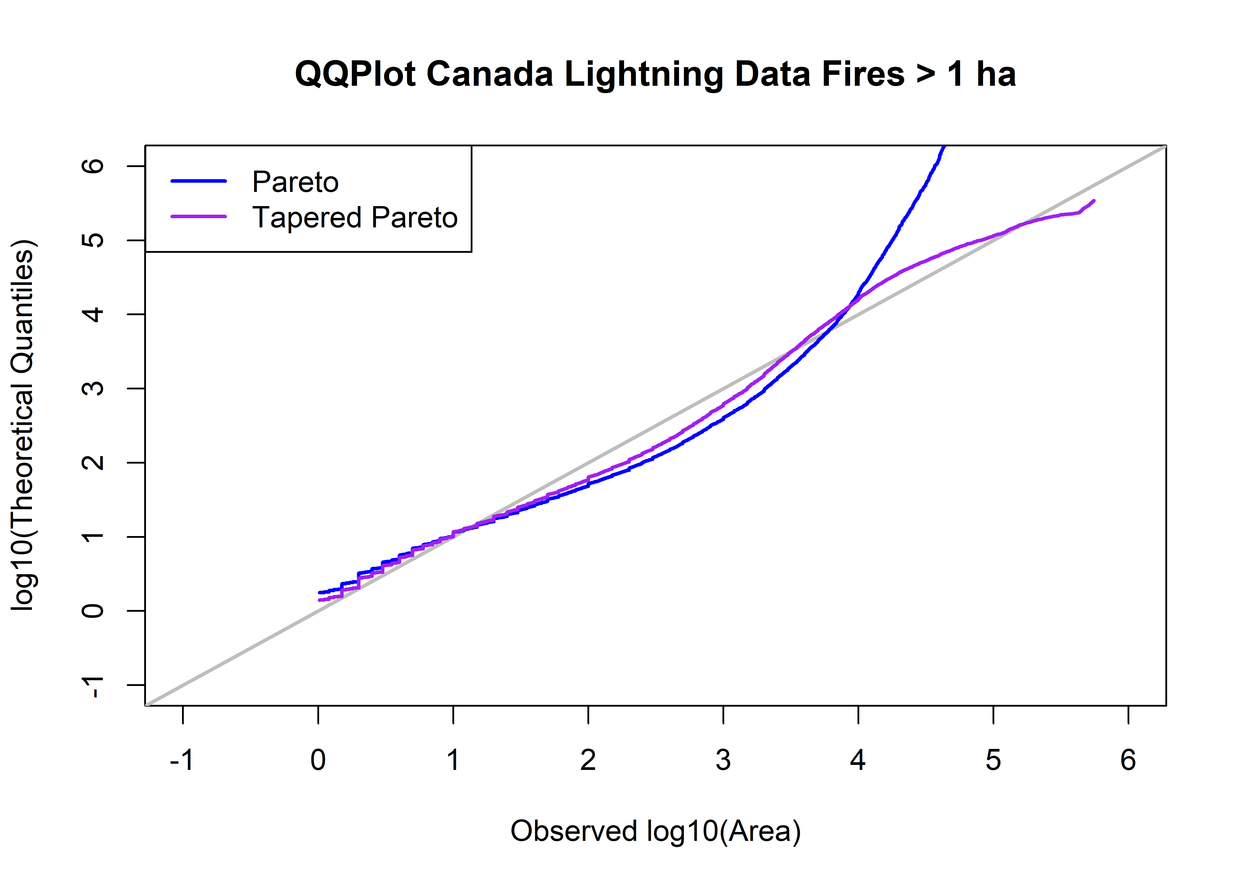
5.3 US & Canada Data
Get lightning data.
uscan.lt <- uscan[uscan$cause1 == 1,]5.3.1 Rank and survival-curve data
Note that this overwrites previous data…
area.thresh = 1.0 # ha
uscan.lt.area <- uscan.lt$area_ha[uscan.lt$area_ha > area.thresh]
uscan.lt.name <- "U.S. & Canada Lightning Data"
uscan.lt.area.max <- max(uscan.lt.area); uscan.lt.area.min <- min(uscan.lt.area)
uscan.lt.nfires <- length(uscan.lt.area)
cbind(uscan.lt.area.max, uscan.lt.area.min, uscan.lt.nfires)
## uscan.lt.area.max uscan.lt.area.min uscan.lt.nfires
## [1,] 553680 1.003621 96700uscan.lt.area.index <- order(uscan.lt.area, na.last=FALSE)
head(uscan.lt.area.index); tail(uscan.lt.area.index)## [1] 48250 50339 60490 31112 1 26## [1] 82945 82955 87554 96275 96254 82831Sort the area data, and get survival-curve ordinates.
uscan.lt.area.sort <- uscan.lt.area[uscan.lt.area.index]
uscan.lt.area.rank <- seq(uscan.lt.nfires, 1)
uscan.lt.area.surv <- uscan.lt.area.rank/uscan.lt.nfires
head(cbind(uscan.lt.area.sort, uscan.lt.area.rank, uscan.lt.area.surv))
## uscan.lt.area.sort uscan.lt.area.rank uscan.lt.area.surv
## [1,] 1.003621 96700 1.0000000
## [2,] 1.003621 96699 0.9999897
## [3,] 1.003621 96698 0.9999793
## [4,] 1.007668 96697 0.9999690
## [5,] 1.011715 96696 0.9999586
## [6,] 1.011715 96695 0.9999483tail(cbind(uscan.lt.area.sort, uscan.lt.area.rank, uscan.lt.area.surv))## uscan.lt.area.sort uscan.lt.area.rank uscan.lt.area.surv
## [96695,] 428100.0 6 6.204757e-05
## [96696,] 438000.0 5 5.170631e-05
## [96697,] 453144.0 4 4.136505e-05
## [96698,] 466420.3 3 3.102378e-05
## [96699,] 501689.1 2 2.068252e-05
## [96700,] 553680.0 1 1.034126e-055.3.2 Initial fits
Plot the observed survivor curve (in red) and that estimated by the Pareto and tapered-Pareto distributions, using guesses of the parameter values.
# Initital values of parameters
a0 <- area.thresh
beta0 <- 0.40
theta0 <-  30000.0

plot(log10(uscan.lt.area.sort), log10(uscan.lt.area.surv),
  type="l", pch=16, cex=0.5, lwd=2, col="red", xlim=c(-1,6), ylim=c(-6,0),
  xlab="log10(Area)", ylab="log10(S(x)", main=paste(uscan.lt.name,"Fires >",as.character(a0),"ha"))
abline(0, -0.5, col="gray", lwd=2)

uscan.lt.fx.pareto <- 1.0 - (a0/uscan.lt.area.sort)^beta0
head(uscan.lt.fx.pareto); tail(uscan.lt.fx.pareto)
## [1] 0.001444851 0.001444851 0.001444851 0.003050892 0.004647929 0.004647929## [1] 0.9944104 0.9944613 0.9945361 0.9945988 0.9947540 0.9949569points(log10(uscan.lt.area.sort), log10(1.0 - uscan.lt.fx.pareto), col="blue", type="l", lwd=2)
uscan.lt.fx.tappareto <- 1.0 - ((a0/uscan.lt.area.sort)^beta0)*exp((a0-uscan.lt.area.sort)/theta0)
head(uscan.lt.fx.tappareto); tail(uscan.lt.fx.tappareto)## [1] 0.001444971 0.001444971 0.001444971 0.003051147 0.004648318 0.004648318## [1] 1 1 1 1 1 1points(log10(uscan.lt.area.sort), log10(1.0 - uscan.lt.fx.tappareto), type="l", pch=16, cex=0.5, col="purple", lwd=2)
legend("bottomleft", title="by hand", legend=c("Observed","Pareto","Tapered Parto",
"slope = -0.5"), lwd=2, col=c("red","blue","purple","gray"))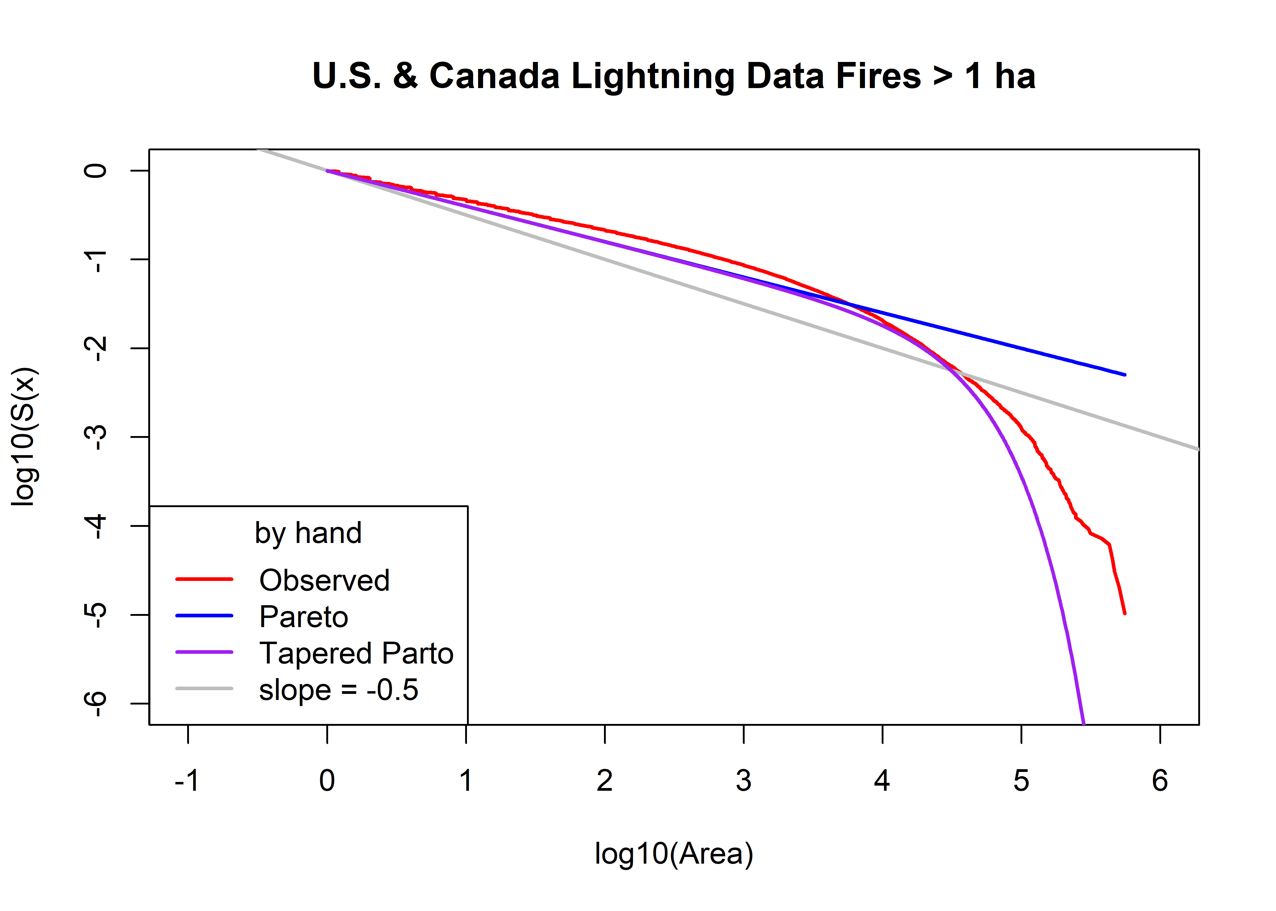
5.3.3 Optimization
# optim() estimation Pareto
SSE.Pareto <- function(p, data, surv){
  y <- log10(surv)
  yhat <- log10((p[2]/data)^p[1])
  x <- sum((y-yhat)^2.0)
  return(x)
}
p0 <- c(beta0, a0); p0
## [1] 0.4 1.0#data=farea; surv=farea.surv
fit.Pareto <- optim(p0, SSE.Pareto, data=uscan.lt.area.sort, surv=uscan.lt.area.surv )
beta1 <- fit.Pareto$par[1]; a1 <- fit.Pareto$par[2]; sse1 <- fit.Pareto$value
beta1; a1; sse1## [1] 0.3981119## [1] 1.346777## [1] 746.8457# optim() estimation tapered Pareto
SSE.tapPareto <- function(p, data, surv){
y <- log10(surv)
yhat <- log10(((p[3]/data)^p[1])*exp((p[3]-data)/p[2]))
x <- sum((y-yhat)^2.0)
return(x)
}
p2 <- c(beta0, theta0, a0); p2## [1] 4e-01 3e+04 1e+00fit.tapPareto1 <- optim(p2, SSE.tapPareto, data=uscan.lt.area.sort, surv=uscan.lt.area.surv)
beta2 <- fit.tapPareto1$par[1]; theta2 <- fit.tapPareto1$par[2]
a2 <- fit.tapPareto1$par[3]; sse2 <- fit.tapPareto1$value
beta2; theta2; a2; sse2## [1] 0.370572## [1] 43140.94## [1] 1.189148## [1] 191.6076# optim() estimation tapered Pareto -- a fixed
SSE.tapPareto2 <- function(p, data, surv, a){
y <- log10(surv)
yhat <- log10( ((a/data)^p[1])*exp((a-data)/p[2]) )
x <- sum((y-yhat)^2.0)
return(x)
}
p3 <- c(beta0, theta0); p3; a <- a0## [1] 4e-01 3e+04fit.tapPareto2 <- optim(p3, SSE.tapPareto2, data=uscan.lt.area.sort, a=a, surv=uscan.lt.area.surv)
beta3 <- fit.tapPareto2$par[1]; theta3 <- fit.tapPareto2$par[2]
a3 <- a0; sse3 <- fit.tapPareto2$value
beta3; theta3; a3; sse3## [1] 0.3568085## [1] 41129.24## [1] 1## [1] 222.7387# compare observed and fitted
plot(log10(uscan.lt.area.sort), log10(uscan.lt.area.surv), type="n", ylim=c(-5,0), xlim=c(-1,6),
xlab="log10(Area)", ylab="log10(S(x)", main=paste(uscan.lt.name,"Fires >",as.character(a0),"ha"))
abline(log10(uscan.lt.area.min)/2, -0.5, col="gray", lwd=2)
uscan.lt.fx.pareto <- 1.0 - (a1/uscan.lt.area.sort)^beta1
head(uscan.lt.fx.pareto); tail(uscan.lt.fx.pareto)## [1] -0.1242144 -0.1242144 -0.1242144 -0.1224148 -0.1206252 -0.1206252## [1] 0.9935511 0.9936095 0.9936954 0.9937674 0.9939457 0.9941788points(log10(uscan.lt.area.sort), log10(1.0 - uscan.lt.fx.pareto), col="blue", type="l", lwd=2)
uscan.lt.fx.tappareto <- 1.0 - ((a2/uscan.lt.area.sort)^beta2)*exp((a2-uscan.lt.area.sort)/theta2)
head(uscan.lt.fx.tappareto); tail(uscan.lt.fx.tappareto)## [1] -0.06487936 -0.06487936 -0.06487936 -0.06329245 -0.06171426 -0.06171426## [1] 0.9999996 0.9999997 0.9999998 0.9999998 0.9999999 1.0000000points(log10(uscan.lt.area.sort), log10(1.0 - uscan.lt.fx.tappareto), col="purple", type="l", lwd=2)
uscan.lt.fx.tappareto <- 1.0 - ((a3/uscan.lt.area.sort)^beta3)*exp((a3-uscan.lt.area.sort)/theta3)
head(uscan.lt.fx.tappareto); tail(uscan.lt.fx.tappareto)## [1] 0.001289026 0.001289026 0.001289026 0.002722096 0.004147378 0.004147378## [1] 0.9999997 0.9999998 0.9999998 0.9999999 1.0000000 1.0000000points(log10(uscan.lt.area.sort), log10(1.0 - uscan.lt.fx.tappareto), col="pink", type="l", lwd=2)
points(log10(uscan.lt.area.sort), log10(uscan.lt.area.surv), pch=16, cex=0.5, col="red")
legend("bottomleft", title="optim() fit", legend=c("FPA-FOD","Pareto","Tapered Pareto",
"Tapered Pareto (a fixed)", "slope = -0.5"), lwd=2, col=c("red","blue","purple","pink","gray"))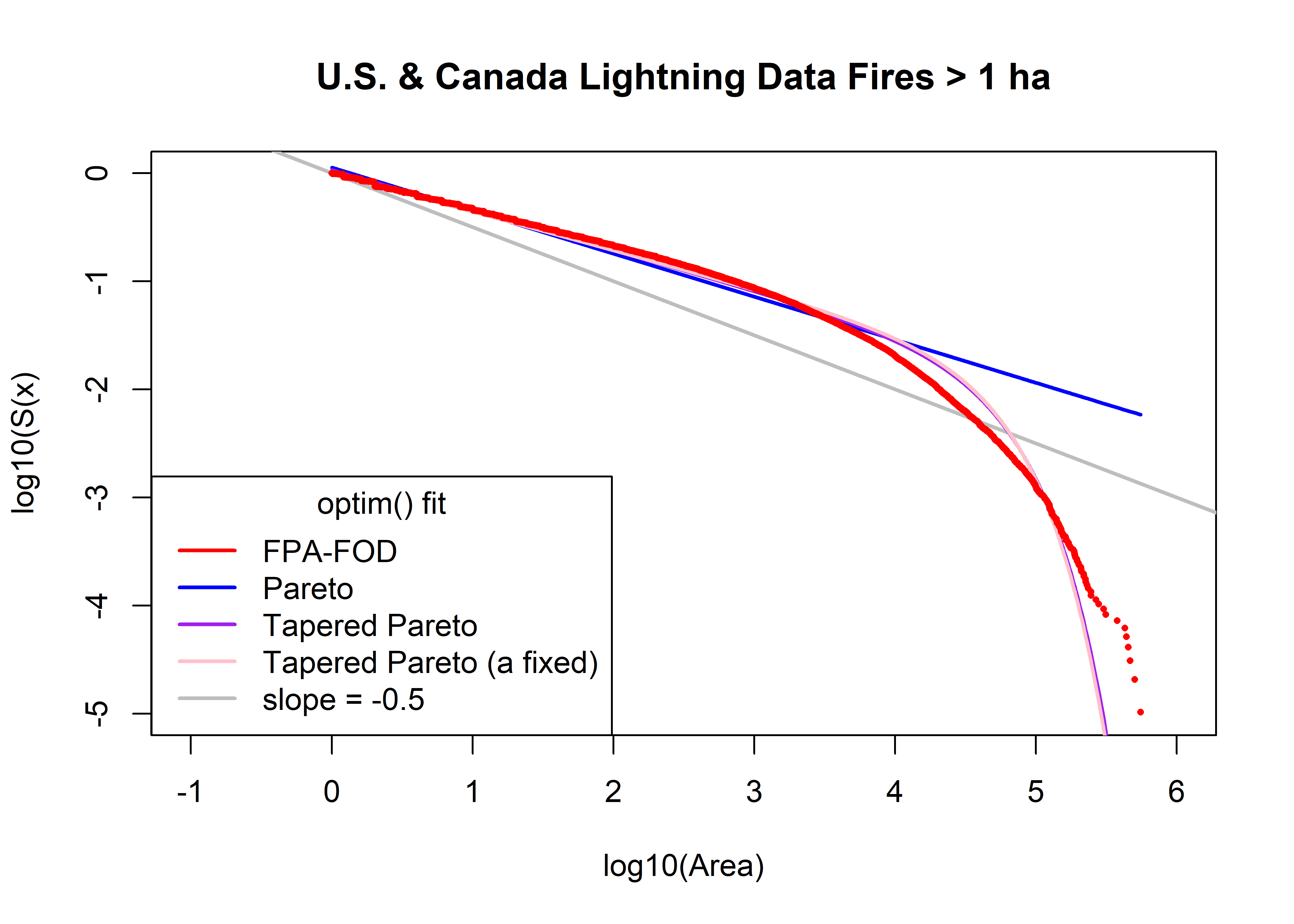
print(cbind(beta0, theta0, a0, beta1, a1, sse1, beta2, theta2, a2, sse2, beta3, theta3, a3, sse3))## beta0 theta0 a0 beta1 a1 sse1 beta2 theta2 a2 sse2 beta3 theta3 a3
## [1,] 0.4 30000 1 0.3981119 1.346777 746.8457 0.370572 43140.94 1.189148 191.6076 0.3568085 41129.24 1
## sse3
## [1,] 222.7387uscan.beta0 <- beta0; uscan.theta0 <- theta0; uscan.a0 <- a0; uscan.beta1 <- beta1; uscan.a1 <- a1;
uscan.beta2 <- beta2; uscan.theta2 <- theta3; uscan.a2 <- a2;
uscan.beta3 <- beta3; uscan.theta3 <- theta3; uscan.a3 <- a35.3.4 QQ Plots
library(PtProcess)
uscan.lt.area.prob <- ppoints(uscan.lt.area.sort)
qp <- qpareto(uscan.lt.area.prob, beta1, a1, lower.tail=TRUE, log.p=FALSE)
head(qp); tail(qp)
## [1] 1.346794 1.346829 1.346864 1.346899 1.346934 1.346969## [1] 6.198498e+10 1.026113e+11 1.929081e+11 4.491621e+11 1.620523e+12 2.559266e+13qtap <- qtappareto(uscan.lt.area.prob, beta2, theta2, a2, lower.tail=TRUE, log.p=FALSE, tol=1e-8)
head(qtap); tail(qtap)## [1] 1.189164 1.189198 1.189231 1.189264 1.189297 1.189330## [1] 227276.8 235374.2 245540.2 259190.9 279994.2 325006.1head(cbind(log10(uscan.lt.area.sort),qp,qtap,log10(qp),log10(qtap),uscan.lt.area.prob))## qp qtap uscan.lt.area.prob
## [1,] 0.001569861 1.346794 1.189164 0.1293013 0.07524187 5.170631e-06
## [2,] 0.001569861 1.346829 1.189198 0.1293125 0.07525399 1.551189e-05
## [3,] 0.001569861 1.346864 1.189231 0.1293238 0.07526611 2.585315e-05
## [4,] 0.003317527 1.346899 1.189264 0.1293351 0.07527823 3.619442e-05
## [5,] 0.005058189 1.346934 1.189297 0.1293464 0.07529035 4.653568e-05
## [6,] 0.005058189 1.346969 1.189330 0.1293577 0.07530247 5.687694e-05tail(cbind(log10(uscan.lt.area.sort),qp,qtap,log10(qp),log10(qtap),uscan.lt.area.prob))## qp qtap uscan.lt.area.prob
## [96695,] 5.631545 6.198498e+10 227276.8 10.79229 5.356555 0.9999431
## [96696,] 5.641474 1.026113e+11 235374.2 11.01120 5.371759 0.9999535
## [96697,] 5.656236 1.929081e+11 245540.2 11.28535 5.390123 0.9999638
## [96698,] 5.668777 4.491621e+11 259190.9 11.65240 5.413620 0.9999741
## [96699,] 5.700435 1.620523e+12 279994.2 12.20966 5.447149 0.9999845
## [96700,] 5.743259 2.559266e+13 325006.1 13.40812 5.511892 0.9999948plot(log10(uscan.lt.area.sort), log10(qtap), xlim=c(-1,6), ylim=c(-1,6), xlab="Observed log10(Area)", type="n",
ylab="log10(Theoretical Quantiles)", main=paste("QQPlot",uscan.lt.name,"Fires >",as.character(a0),"ha"))
abline(0.0, 1.0, col="gray", lwd=2)
points(log10(uscan.lt.area.sort),log10(qp), type="l", col="blue", lwd=2)
points(log10(uscan.lt.area.sort),log10(qtap), type="l", col="purple", lwd=2)
legend("topleft", legend=c("Pareto","Tapered Pareto"), lwd=2, col=c("blue","purple"))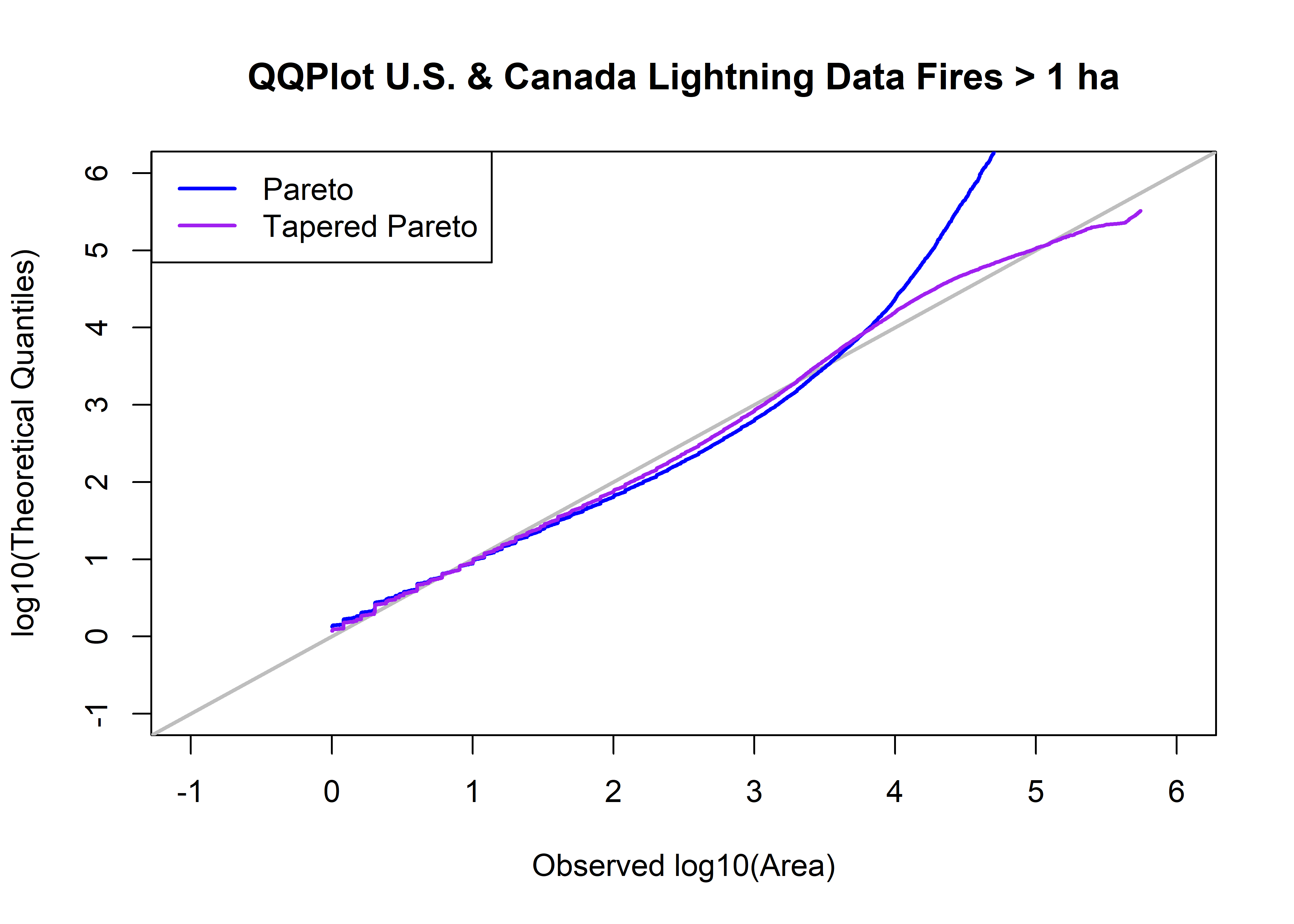
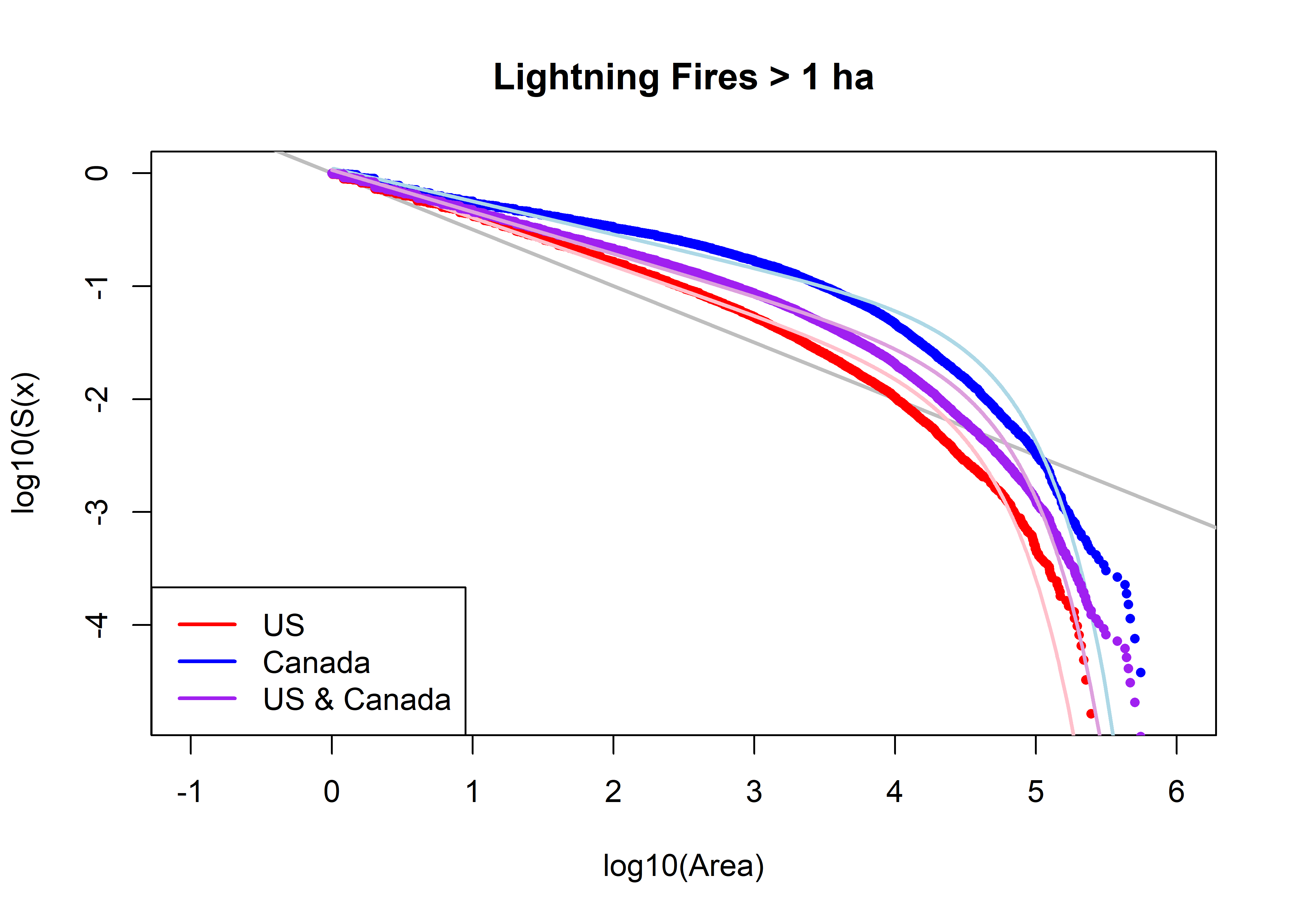
5.4 Compare Tapered-Pareto Fits
# compare observed and fitted
plot(log10(fpafod.lt.area.sort), log10(fpafod.lt.area.surv), xlab="log10(Area)", ylab="log10(S(x)", type="n",
  xlim=c(-1,6), main=paste("Lightning Fires >",as.character(a0),"ha"))
abline(log10(fpafod.lt.area.min)/2, -0.5, col="gray", lwd=2)

points(log10(fpafod.lt.area.sort), log10(fpafod.lt.area.surv), col="red", pch=16, cex=0.7 )
fpafod.lt.fx.tappareto <- 1.0 - ((us.a2/fpafod.lt.area.sort)^us.beta2)*exp((us.a2-fpafod.lt.area.sort)/
    us.theta2)
points(log10(fpafod.lt.area.sort), log10(1.0 - fpafod.lt.fx.tappareto), col="pink", type="l", lwd=2)

points(log10(cnfdb.lt.area.sort), log10(cnfdb.lt.area.surv), col="blue", pch=16, cex=0.7)
cnfdb.lt.fx.tappareto <- 1.0 - ((can.a2/cnfdb.lt.area.sort)^can.beta2)*exp((can.a2-cnfdb.lt.area.sort)/
    can.theta2)
points(log10(cnfdb.lt.area.sort), log10(1.0 - cnfdb.lt.fx.tappareto), col="lightblue", type="l", lwd=2)

points(log10(uscan.lt.area.sort), log10(uscan.lt.area.surv), col="purple", pch=16, cex=0.7)
uscan.lt.fx.tappareto <- 1.0 - ((uscan.a2/uscan.lt.area.sort)^uscan.beta2)*exp((uscan.a2-uscan.lt.area.sort)/
    uscan.theta2)
points(log10(uscan.lt.area.sort), log10(1.0 - uscan.lt.fx.tappareto), col="plum", type="l", lwd=2)
legend("bottomleft", legend=c("US","Canada","US & Canada"), lwd=2, col=c("red","blue", "purple"))