National Fire Occurrence Data (NFO)
1 National Fire Occurrence Data, Federal and State Lands, 1986-1996, v1999
National Fire Occurrence Data, Federal and State Lands, 1986-1996, v1999 – http://www.firelab.org/document/national-fire-occurrence-federal-and-state-lands-1986-1996-v1999 (This is the current name and location of these data– they were formerlly called the National Fire Occurrence Database.)
1.1 Overview
Because the current version of the file stptfire.shp_.zip (and the component .dbf file) is damaged, the cleaned-up data set originally developed by Sarah Shafer was used. The basic take-away message here is that these data are fine, but are limited in time (1986-1996) and space (coterminous U.S. only).
Read the data.
filename <- "e:/Projects/fire/DailyFireStarts/data/NFOv1999/allfireb.csv"
nfo <- read.csv(filename)
List the first and last lines.
head(nfo); tail(nfo)## LAT_DD LONG_DD YEAR MONTH_DISC DAY_DISC MONTH_CONT DAY_CONT HECTARES_TOTAL CAUSE_STD CAUSE2 SOURCE
## 1 48.966 -121.813 1990 8 15 8 24 0.08 1 1 f
## 2 48.932 -121.966 1991 8 26 8 30 1.21 9 2 f
## 3 48.932 -121.949 1991 9 30 10 5 0.36 9 2 f
## 4 48.966 -121.763 1990 8 10 8 24 0.20 1 1 f
## 5 48.949 -121.830 1990 8 10 8 11 0.12 1 1 f
## 6 48.932 -121.763 1990 8 10 8 12 0.12 1 1 f
## UNIQUENUM
## 1 590246307
## 2 591271561
## 3 591271562
## 4 590246304
## 5 590246305
## 6 590246303## LAT_DD LONG_DD YEAR MONTH_DISC DAY_DISC MONTH_CONT DAY_CONT HECTARES_TOTAL CAUSE_STD CAUSE2
## 976027 41.89077 -85.16563 1988 7 6 7 21 0.81 4 2
## 976028 41.85097 -84.14974 1996 8 14 8 27 0.97 4 2
## 976029 41.83451 -84.28418 1988 7 4 7 5 10.12 6 2
## 976030 41.83283 -84.52458 1996 4 18 4 18 1.21 4 2
## 976031 41.76099 -84.20419 1988 6 13 6 13 1.21 4 2
## 976032 41.75822 -84.34524 1991 10 17 10 29 8.90 5 2
## SOURCE UNIQUENUM
## 976027 s 266130
## 976028 s 266213
## 976029 s 266212
## 976030 s 266190
## 976031 s 266206
## 976032 s 266209length(nfo[,1]) # Number of points in the data set## [1] 976032str(nfo, strict.width="cut") # Variables in the data set## 'data.frame': 976032 obs. of 12 variables:
## $ LAT_DD : num 49 48.9 48.9 49 48.9 ...
## $ LONG_DD : num -122 -122 -122 -122 -122 ...
## $ YEAR : int 1990 1991 1991 1990 1990 1990 1991 1989 1993 1995 ...
## $ MONTH_DISC : int 8 8 9 8 8 8 8 9 9 9 ...
## $ DAY_DISC : int 15 26 30 10 10 10 6 28 26 14 ...
## $ MONTH_CONT : int 8 8 10 8 8 8 8 10 10 9 ...
## $ DAY_CONT : int 24 30 5 24 11 12 10 2 4 25 ...
## $ HECTARES_TOTAL: num 0.08 1.21 0.36 0.2 0.12 0.12 0.04 4.86 0.04 0.04 ...
## $ CAUSE_STD : int 1 9 9 1 1 1 1 2 7 9 ...
## $ CAUSE2 : int 1 2 2 1 1 1 1 2 2 2 ...
## $ SOURCE : Factor w/ 3 levels "c","f","s": 2 2 2 2 2 2 2 2 2 2 ...
## $ UNIQUENUM : int 590246307 591271561 591271562 590246304 590246305 590246303 591271554 589246264..Map the data
library(maps)
plot(nfo$LAT_DD ~ nfo$LONG_DD, ylim=c(25,50), xlim=c(-125,-65), type="n",
  xlab="Longitude", ylab="Latitude")
map("world", add=TRUE, lwd=2, col="gray")
map("state", add=TRUE, lwd=2, col="gray")
points(nfo$LAT_DD ~ nfo$LONG_DD, pch=16, cex=0.2, col="red")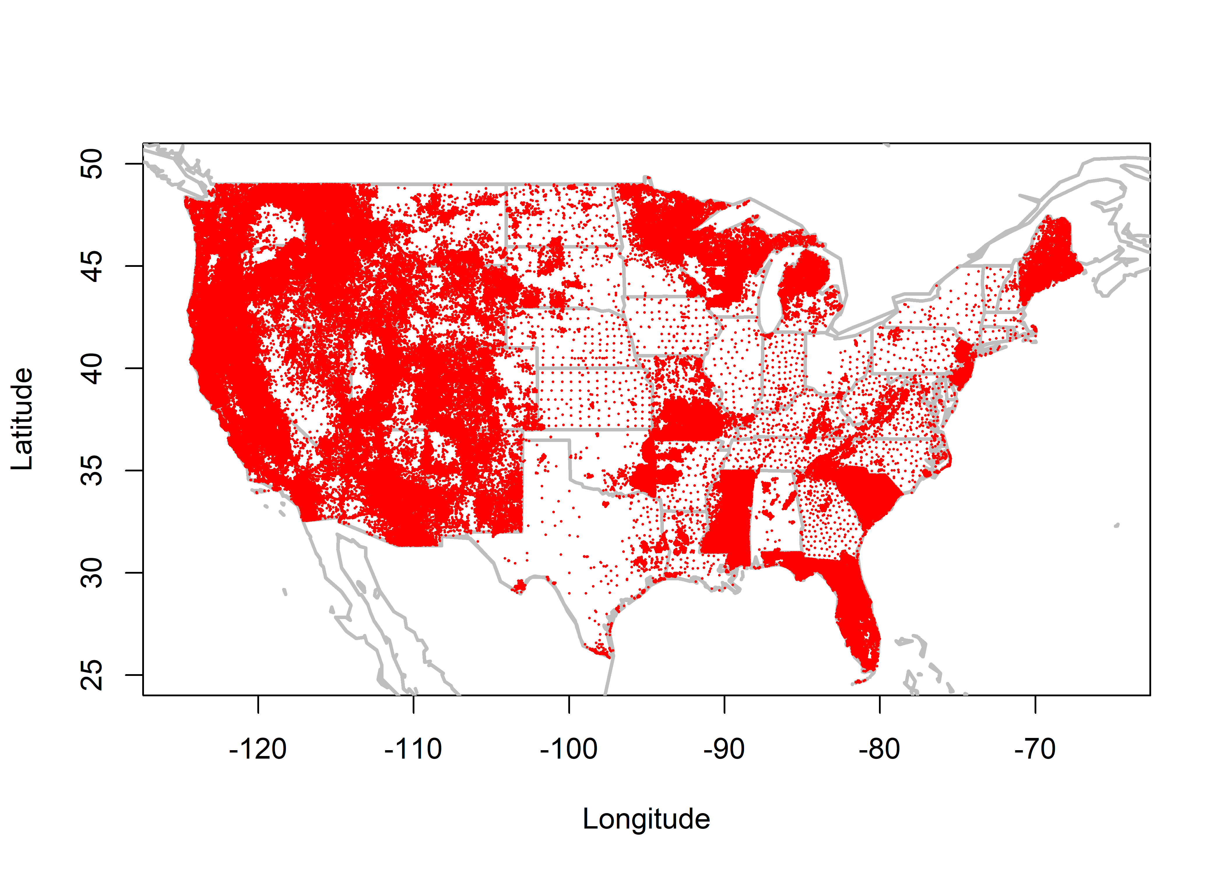
Number of fires by different causes, cause=0 (unknown), cause=1 (lightning), cause=2 (human)
table(nfo$CAUSE2)##
## 0 1 2
## 74541 143796 757695library(lubridate)
nfo$startdate <- as.Date(paste(as.character(nfo$YEAR),as.character(nfo$MONTH_DISC),
as.character(nfo$DAY_DISC), sep="-"))
nfo$startdaynum <- yday((strptime(nfo$startdate, "%Y-%m-%d")))
nfo$startday <- as.numeric(format(nfo$DAY_DISC, format="%d"))
nfo$startmon <- as.numeric(format(nfo$MONTH_DISC, format="%m"))Histograms of start-day number of the YEAR_ (startdaynum) for all data, human and lightning:
hist(nfo$startdaynum, breaks=seq(-0.5,366.5,by=1), freq=-TRUE, ylim=c(0,8000), xlim=c(0,400))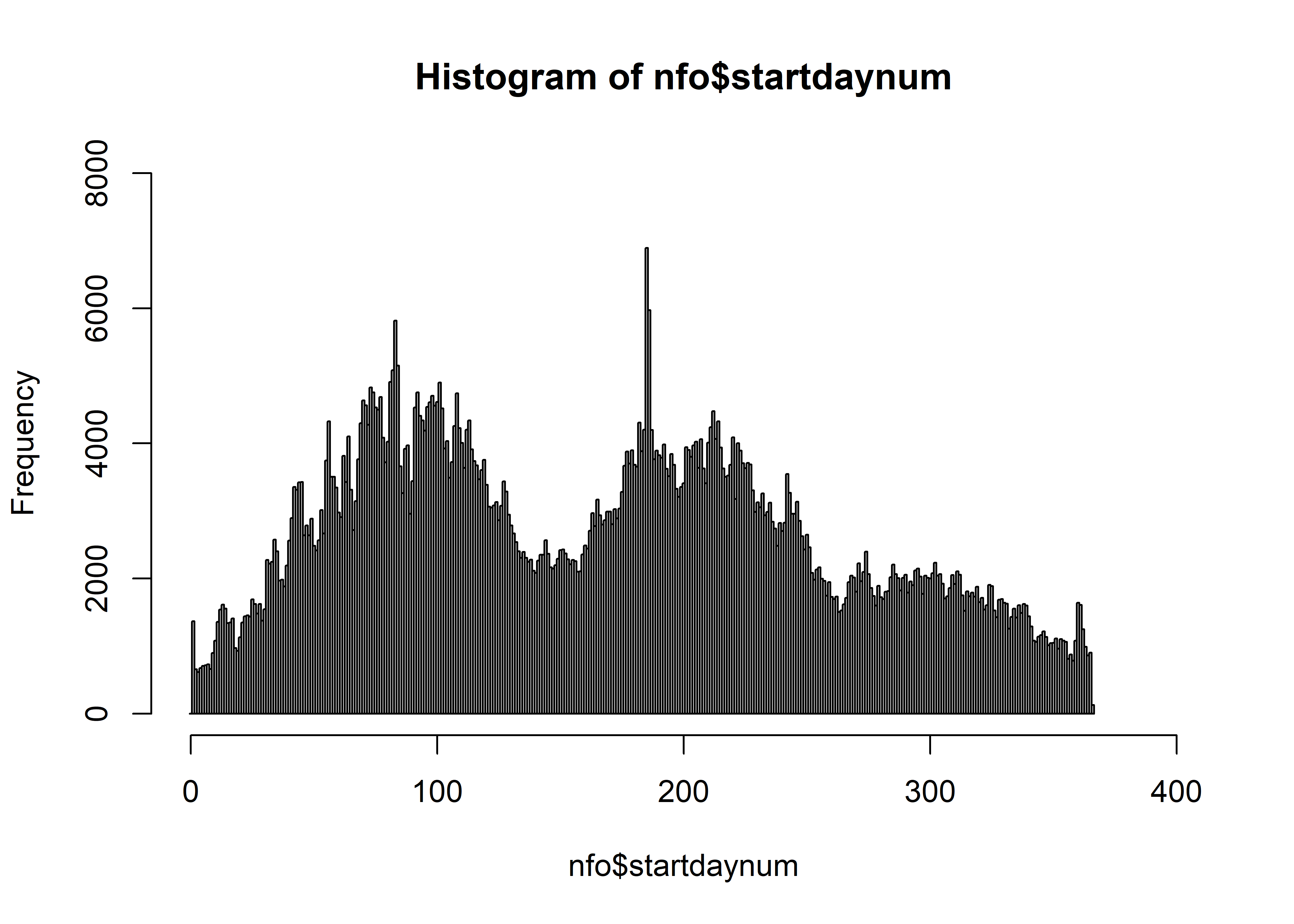
hist(nfo$startdaynum[nfo$CAUSE2==1], breaks=seq(-0.5,366.5,by=1), freq=-TRUE,
  xlim=c(0,400), ylim=c(0,6000), main="nfo Lightning")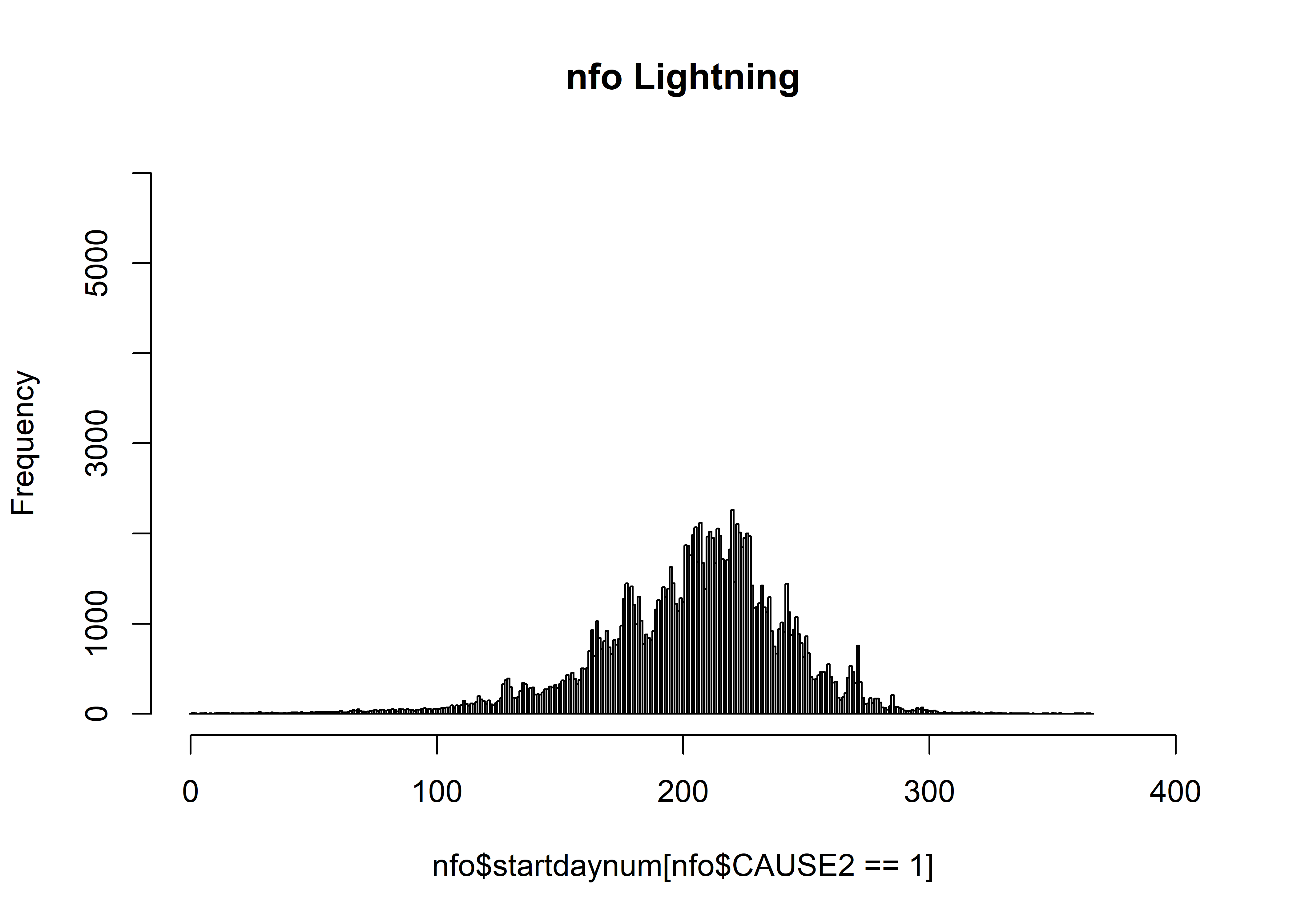
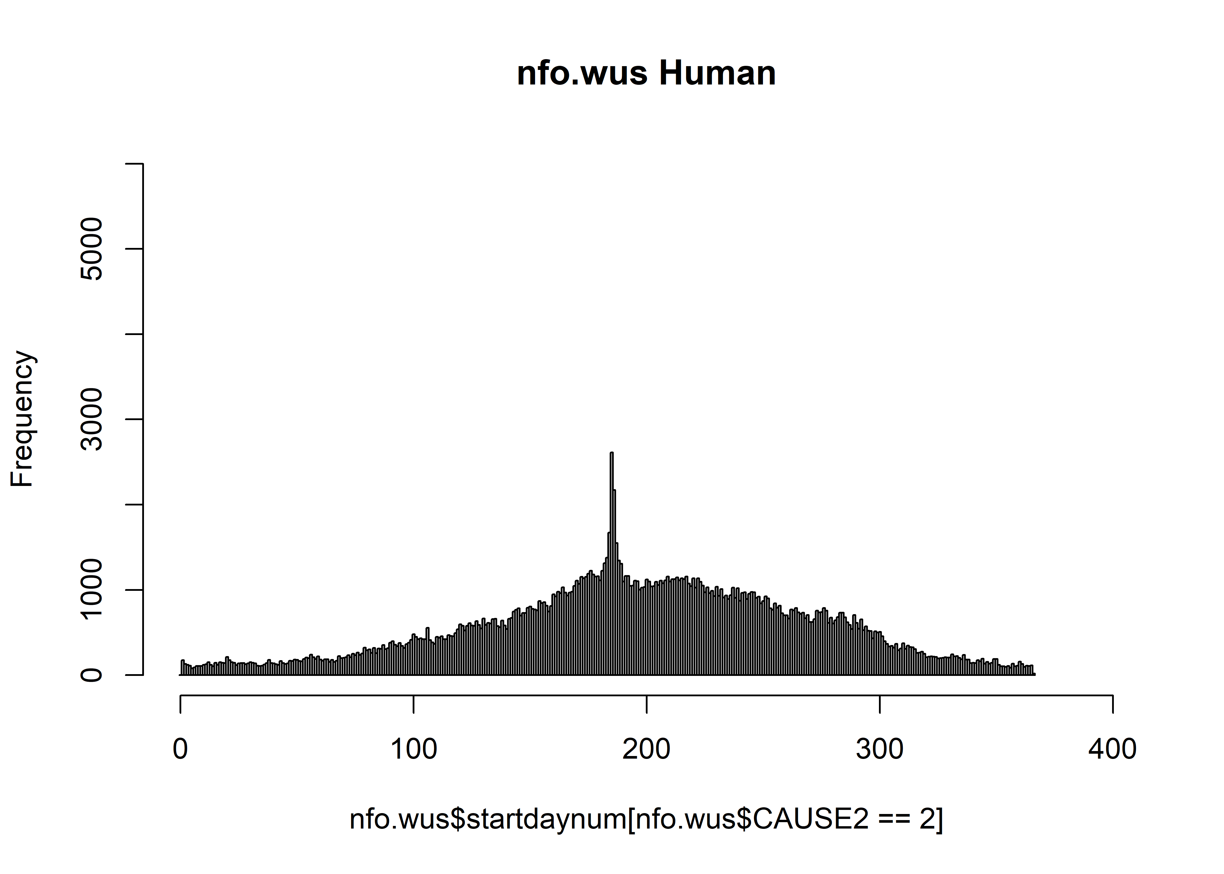
hist(nfo$startdaynum[nfo$CAUSE2==2], breaks=seq(-0.5,366.5,by=1), freq=-TRUE,
  xlim=c(0,400), ylim=c(0,6000), main="nfo Human")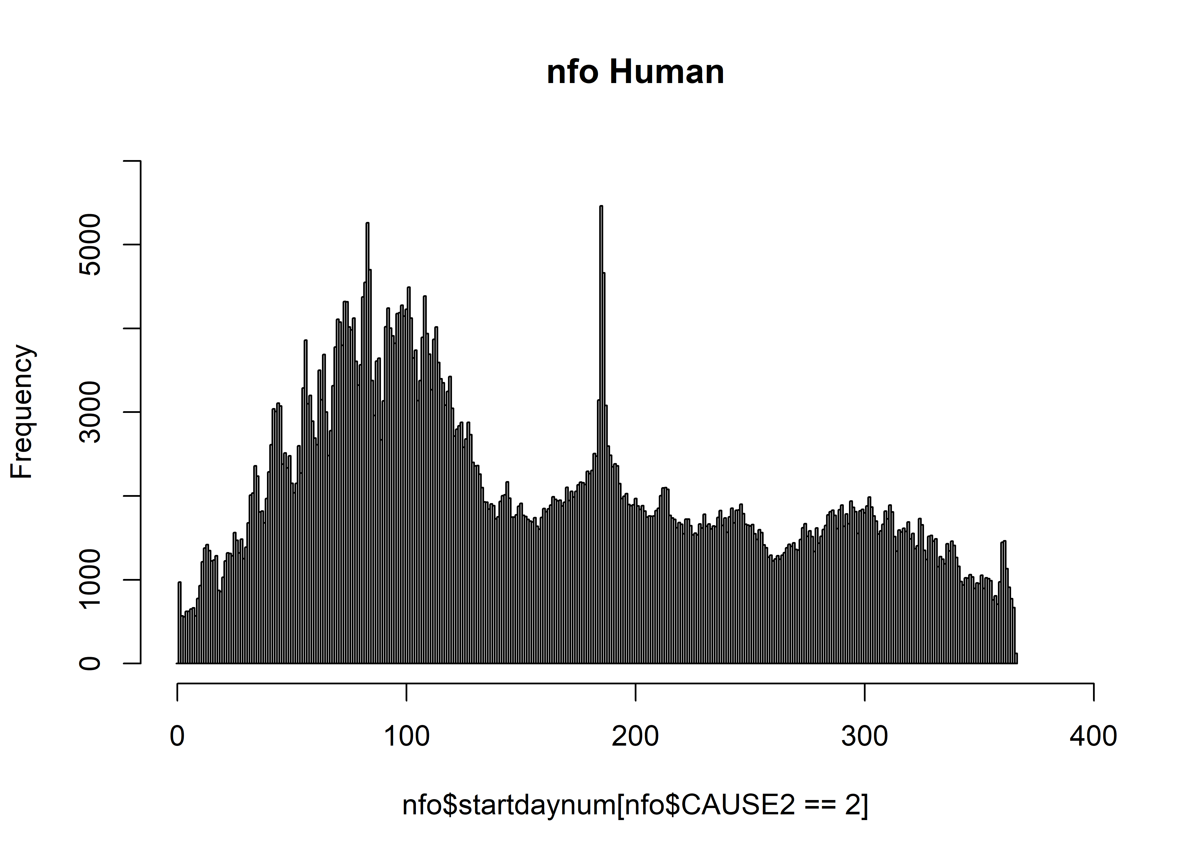
Histograms of the start day over all months
hist(nfo$startday, breaks=seq(-0.5,31.5,by=1), freq=-TRUE, ylim=c(0,60000))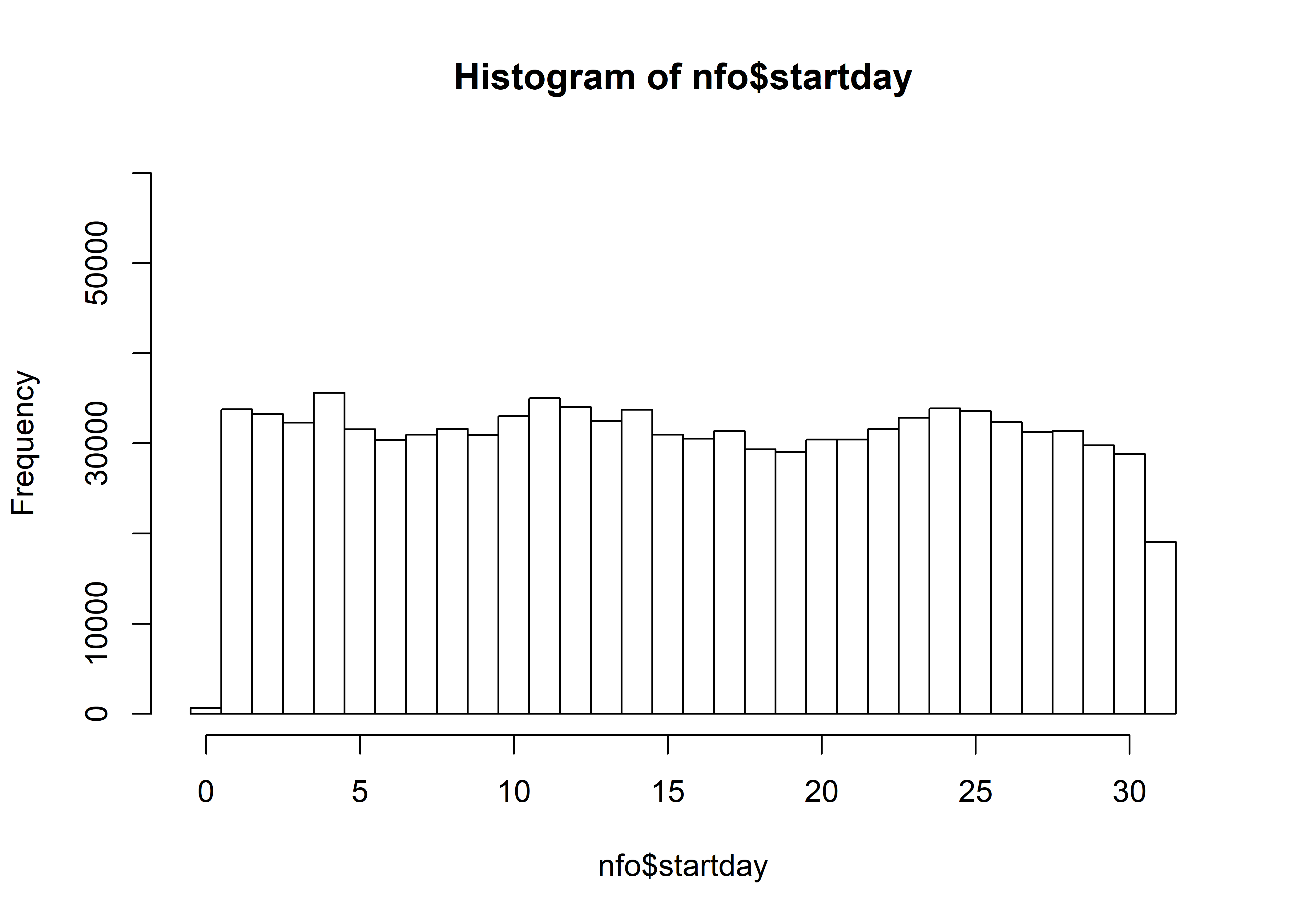
hist(nfo$startday[nfo$CAUSE2==1], breaks=seq(-0.5,31.5,by=1), freq=-TRUE, ylim=c(0,30000),
  main="nfo Lightning")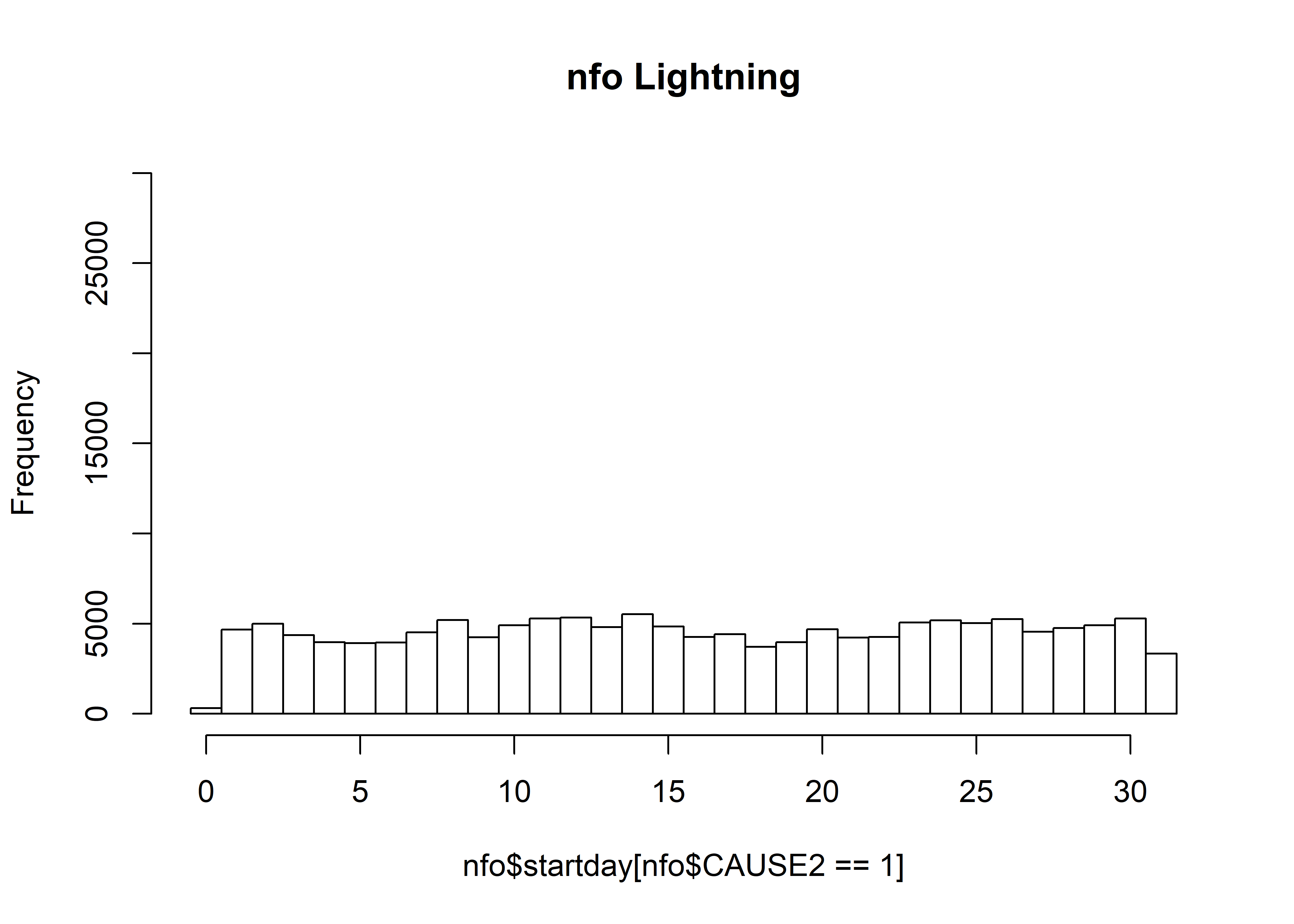
hist(nfo$startday[nfo$CAUSE2==2], breaks=seq(-0.5,31.5,by=1), freq=-TRUE, ylim=c(0,30000),
  main="nfo Human")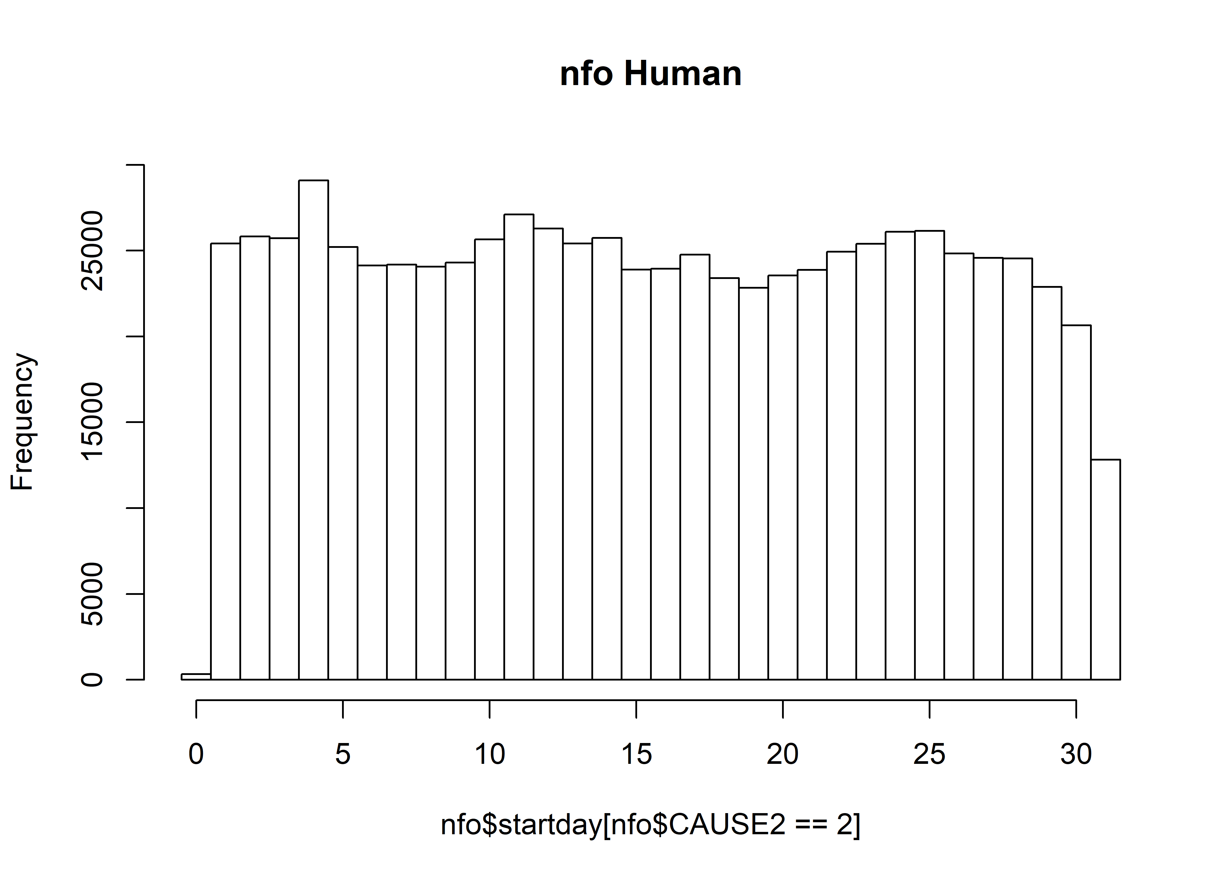
length(nfo$startday)## [1] 976032hist(nfo$startday, breaks=seq(-0.5,31.5,by=1))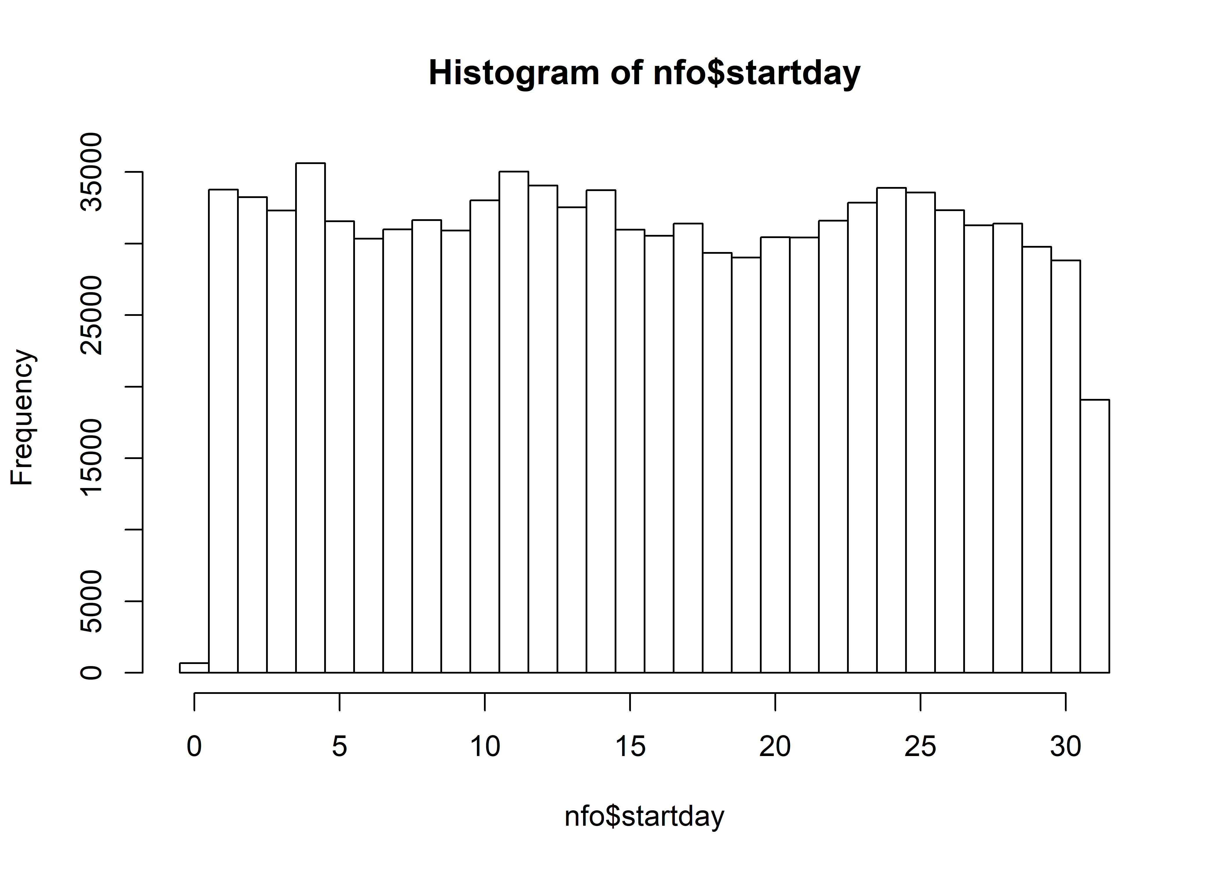
nfo$startday2 <- nfo$startdaynfo$startday2 <- ifelse(nfo$startday2 <= 9, nfo$startday2 <- "1-9", nfo$startday2 <- "10-31")
length(nfo$startday2)## [1] 976032table(nfo$startday2)##
## 1-9 10-31
## 291030 685002nfo.table <- table(nfo$YEAR, nfo$startday2)
nfo.year <- as.integer(row.names(nfo.table))
nfo.ratio <- nfo.table[,1]/nfo.table[,2]
mosaicplot(nfo.table, color=c(3,4), cex.axis=0.6, las=3, main="Start Day in Month by Year")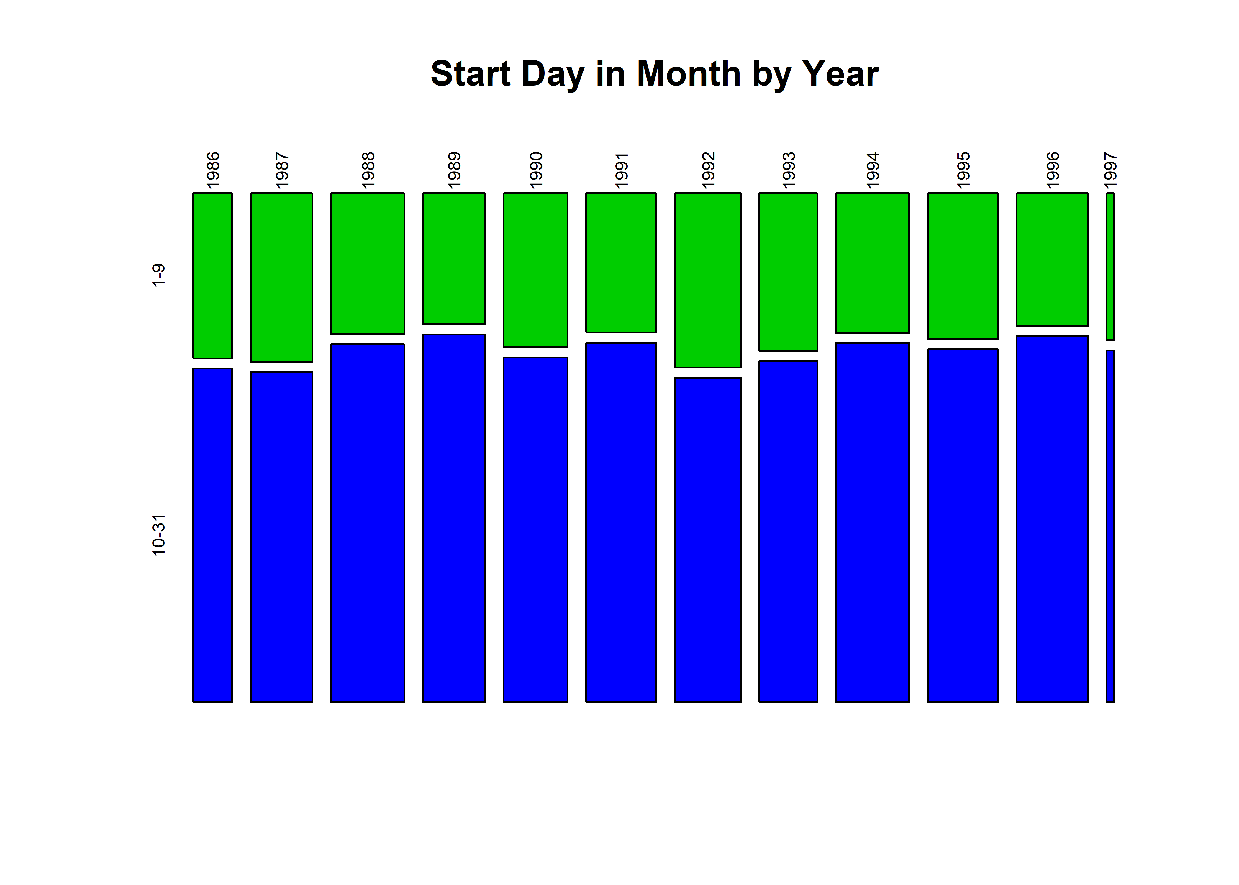
plot(nfo.year, nfo.ratio, pch=16, type="o", lwd=3, col="red")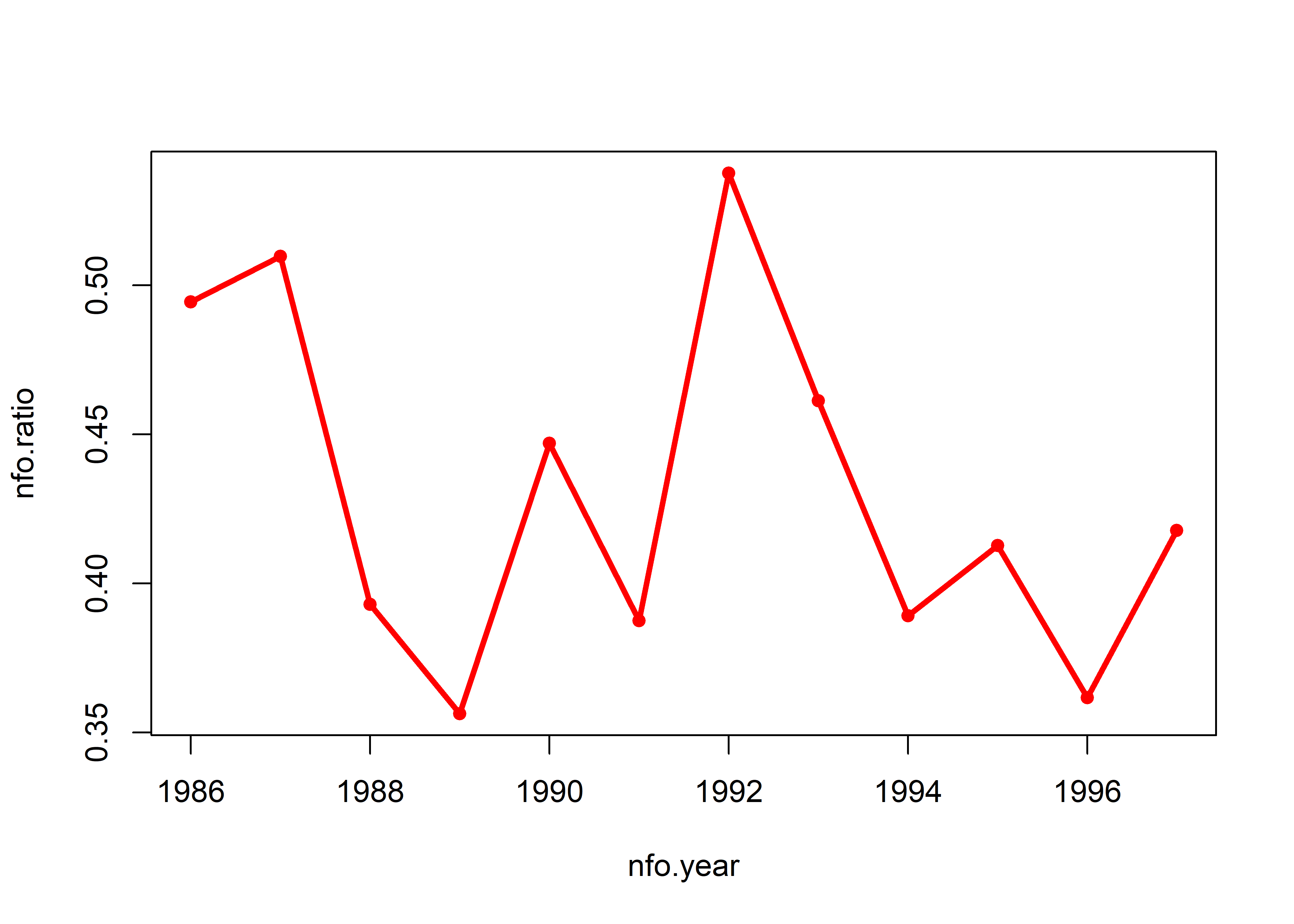
nfo.table.start <- table(nfo$startmon, nfo$startday2)
mosaicplot(nfo.table.start, color=c(3,4), cex.axis=0.6, las=3, main="Start Day in Month by Month")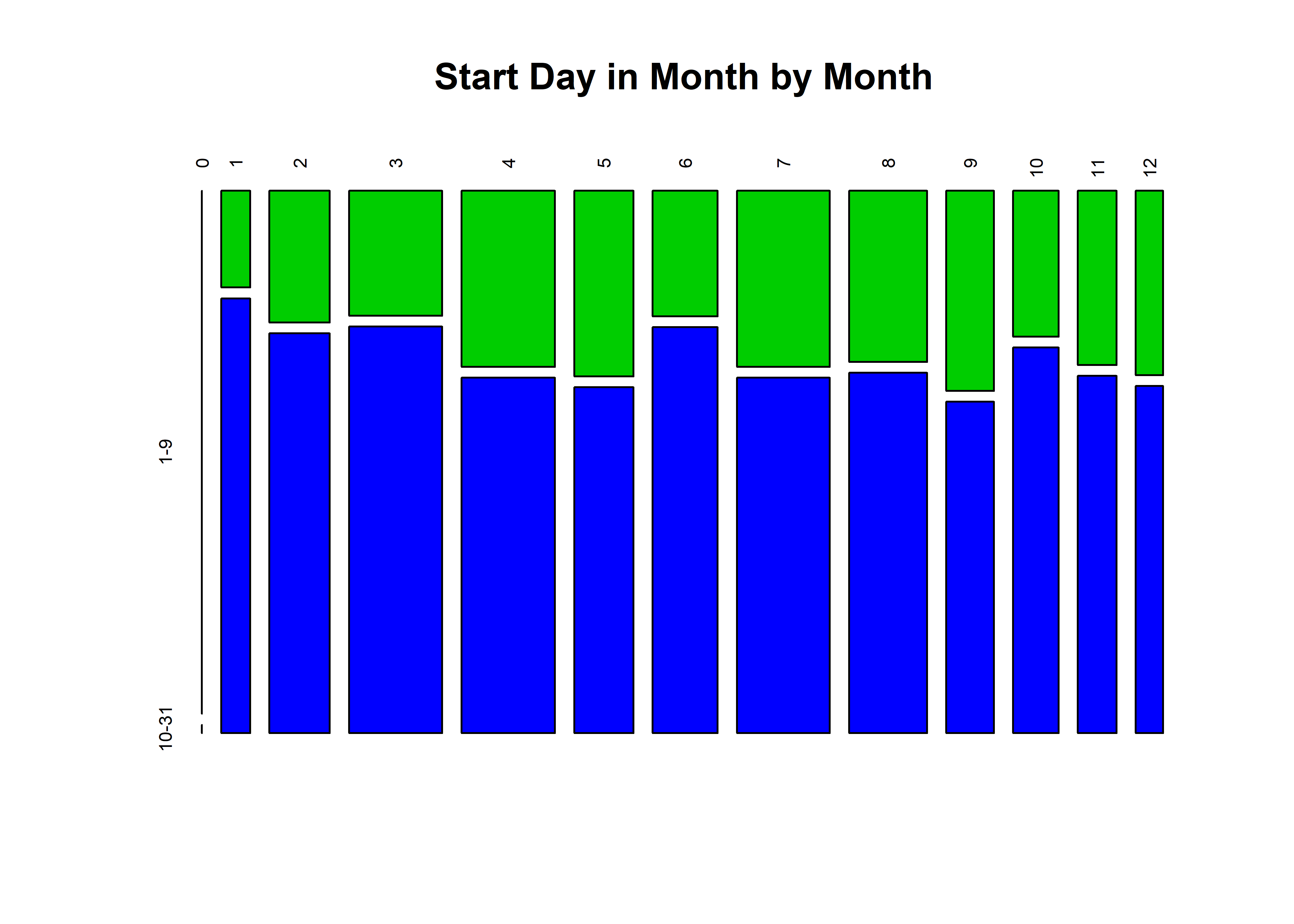
nfo.tablemon <- table(nfo$YEAR, nfo$startmon)
mosaicplot(nfo.tablemon, color=monthcolors, cex.axis=0.6, las=3, main="All Fires")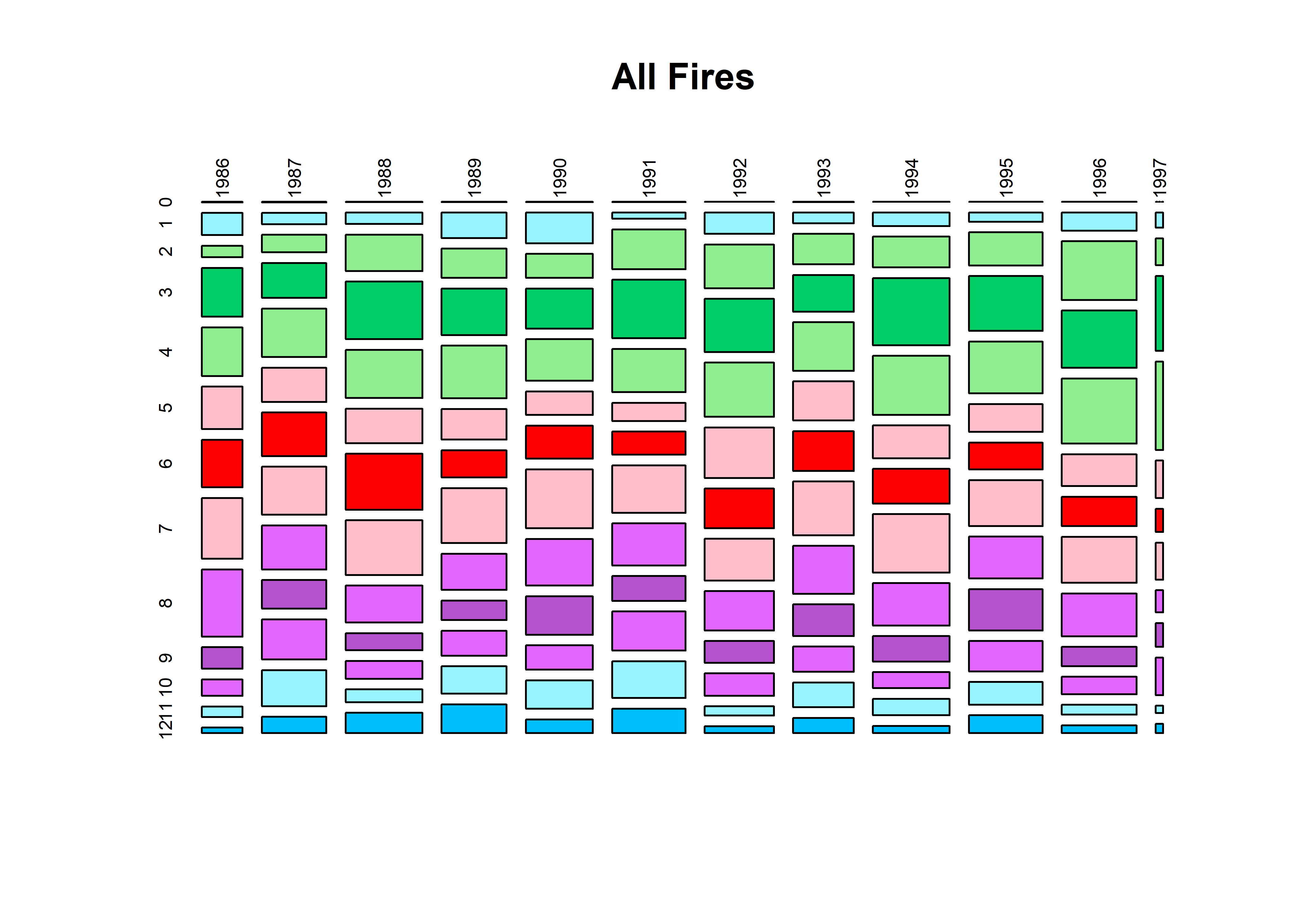
nfo.tablemon.n <- table(nfo$YEAR[nfo$CAUSE2==1], nfo$startmon[nfo$CAUSE2==1])
mosaicplot(nfo.tablemon.n, color=monthcolors, cex.axis=0.6, las=3, main="Lightning Fires")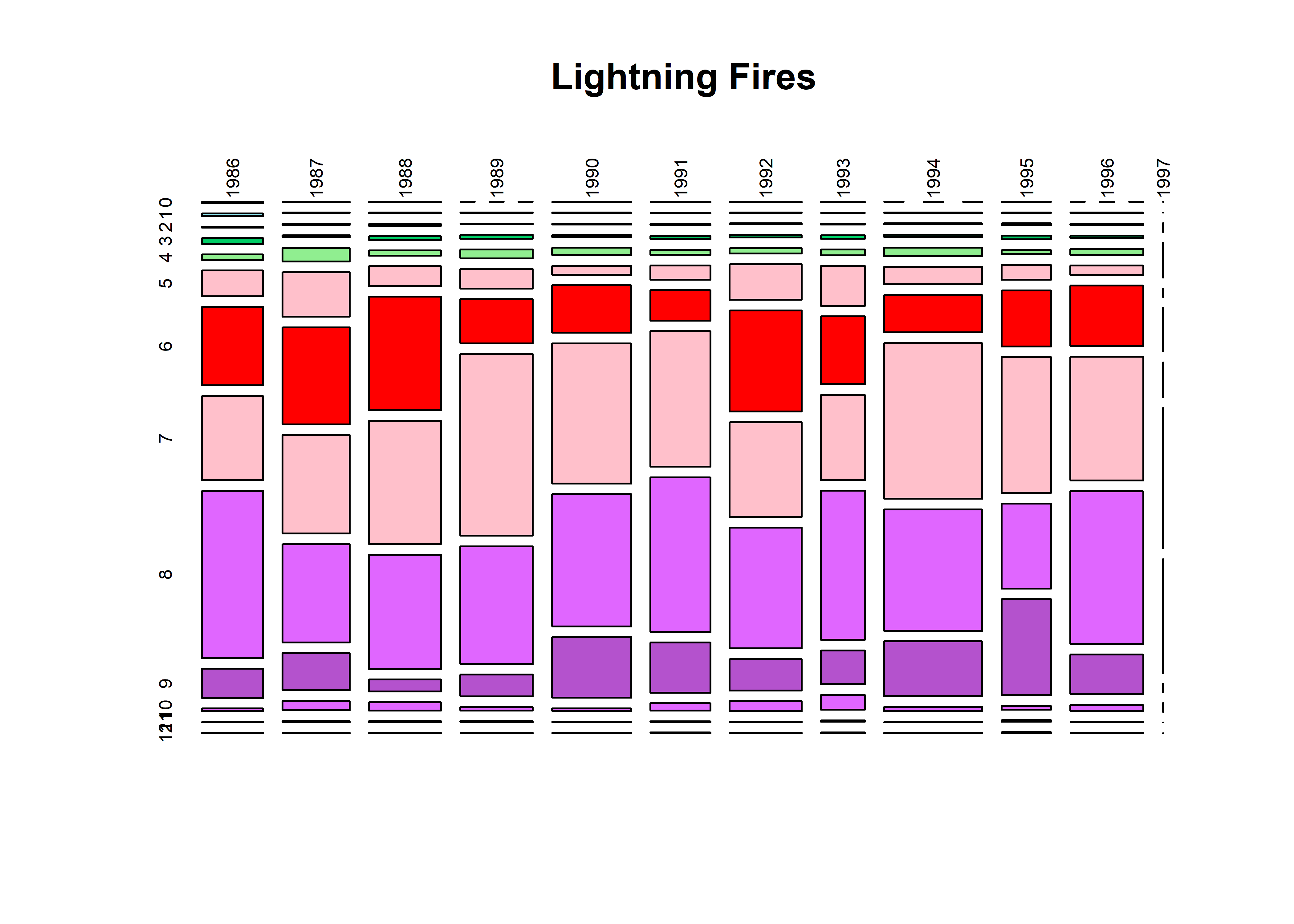
nfo.tablemon.h <- table(nfo$YEAR[nfo$CAUSE2==2], nfo$startmon[nfo$CAUSE2==2])
mosaicplot(nfo.tablemon.h, color=monthcolors, cex.axis=0.6, las=3, main="Human Fires")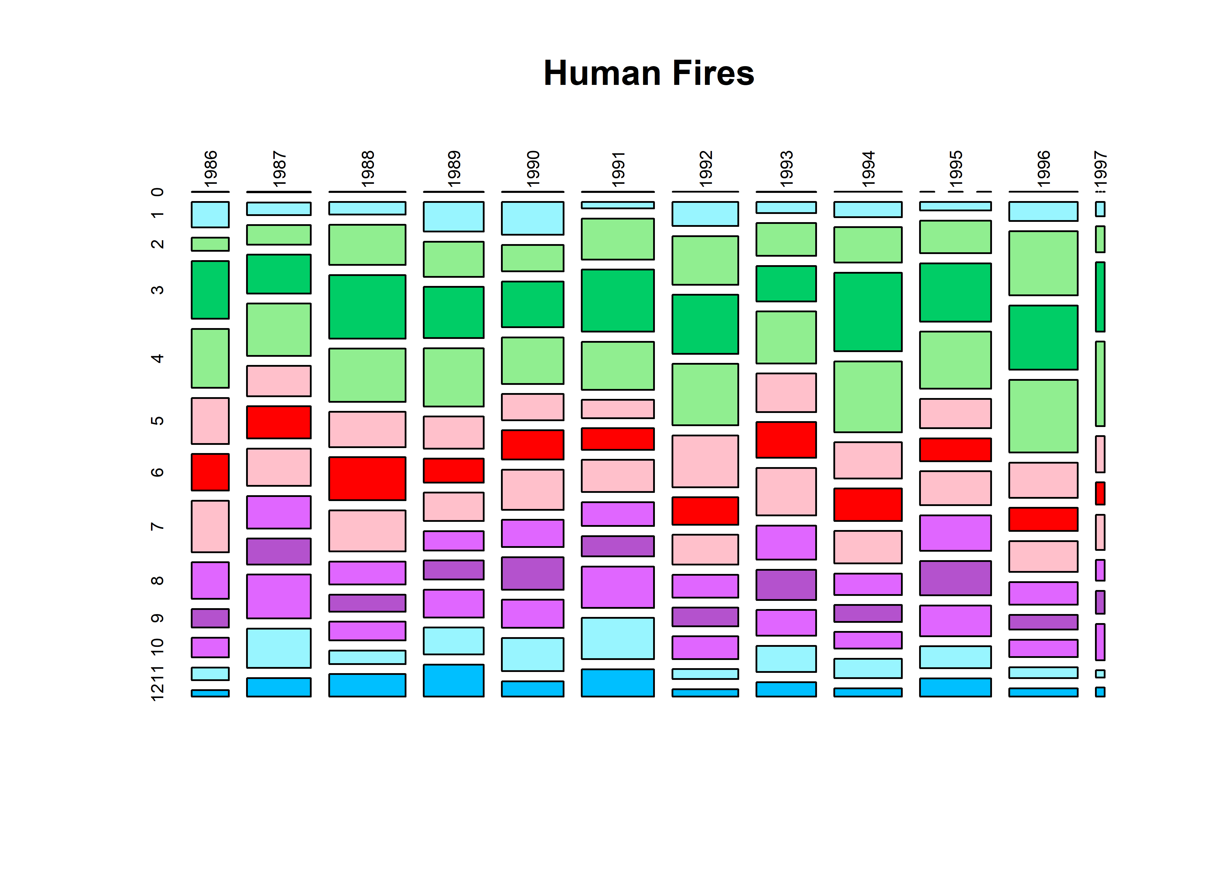
1.2 Western U.S. Subset
This subset should correspond exactly to the data set used in Bartlein et al. (2008) (i.e. fires with longitudes <= -102.0), however, there are few more records
nfo.wus <- nfo[nfo$LONG_DD <= -102.0 & nfo$YEAR <= 1996 ,]
length(nfo.wus[,1])
## [1] 341156table(nfo.wus$CAUSE2)##
## 0 1 2
## 18760 118961 203435Map the data
plot(nfo.wus$LAT_DD ~ nfo.wus$LONG_DD, ylim=c(27.5,50), xlim=c(-125,-100), type="n",
  xlab="Longitude", ylab="Latitude")
map("world", add=TRUE, lwd=2, col="gray")
map("state", add=TRUE, lwd=2, col="gray")
points(nfo.wus$LAT_DD ~ nfo.wus$LONG_DD, pch=16, cex=0.2, col="red")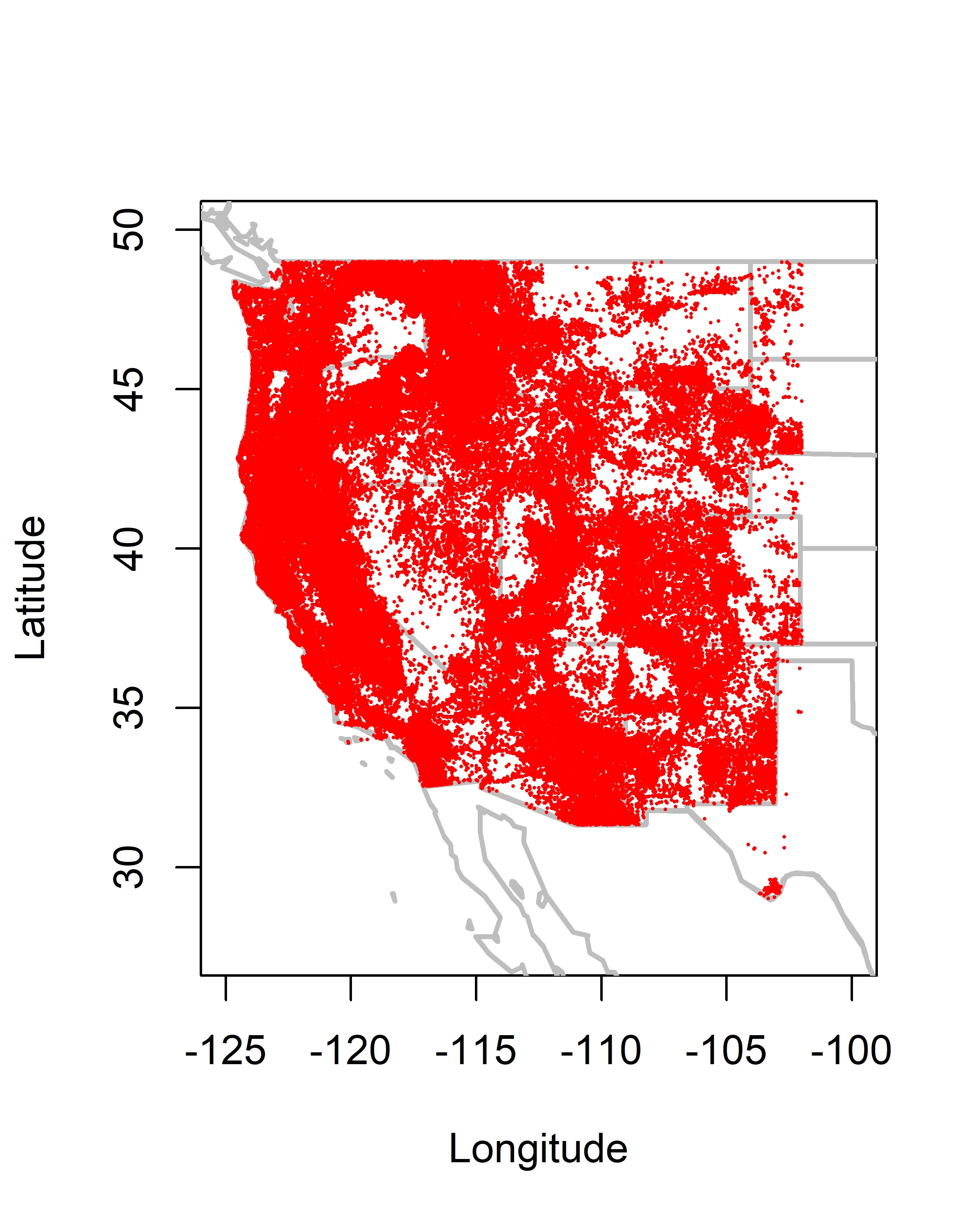
Histograms Western U.S.
hist(nfo.wus$startdaynum, breaks=seq(-0.5,366.5,by=1), freq=-TRUE, ylim=c(0,6000), xlim=c(0,400))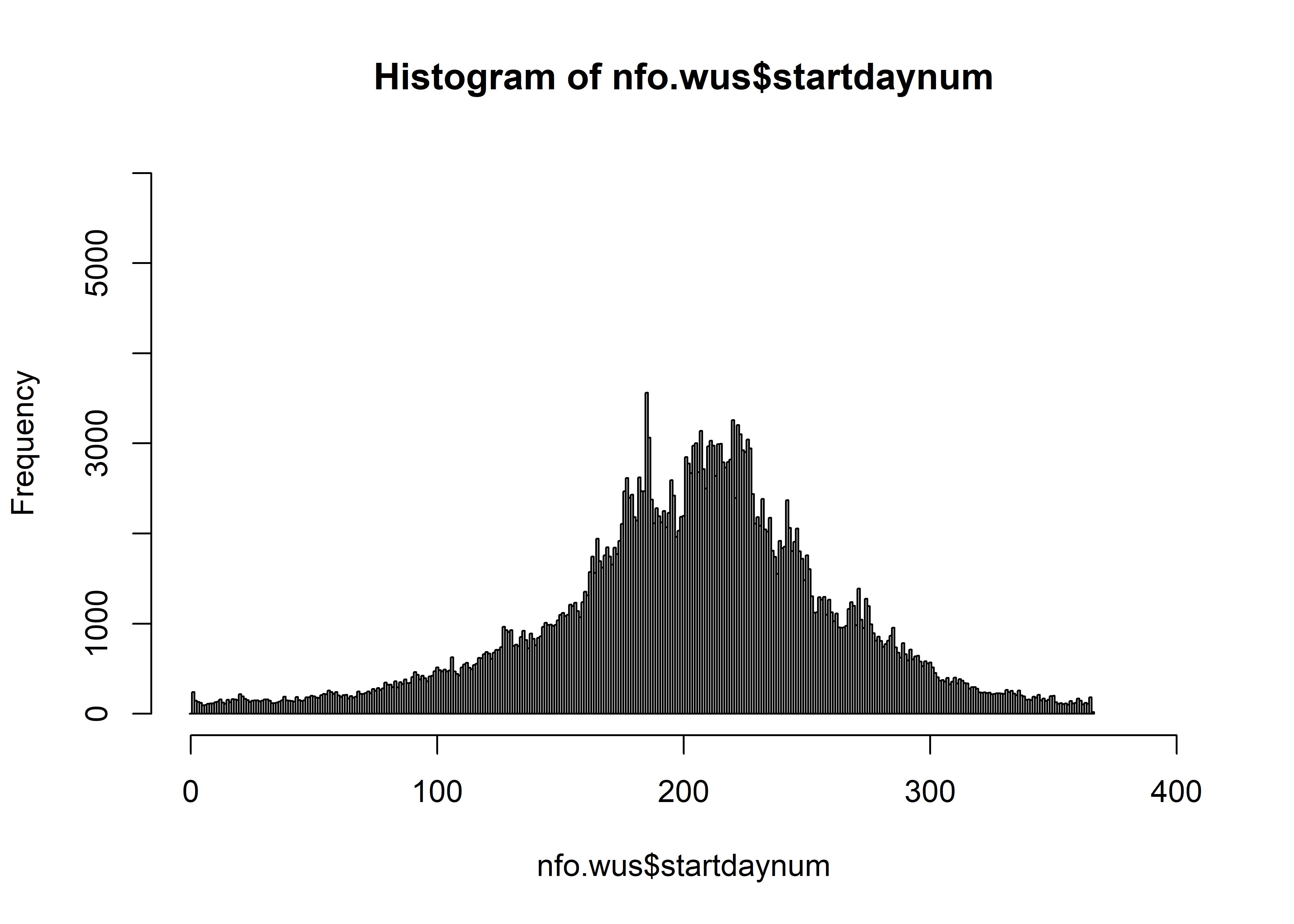
hist(nfo.wus$startdaynum[nfo.wus$CAUSE2==1], breaks=seq(-0.5,366.5,by=1), freq=-TRUE,
  xlim=c(0,400), ylim=c(0,6000), main="nfo.wus Lightning")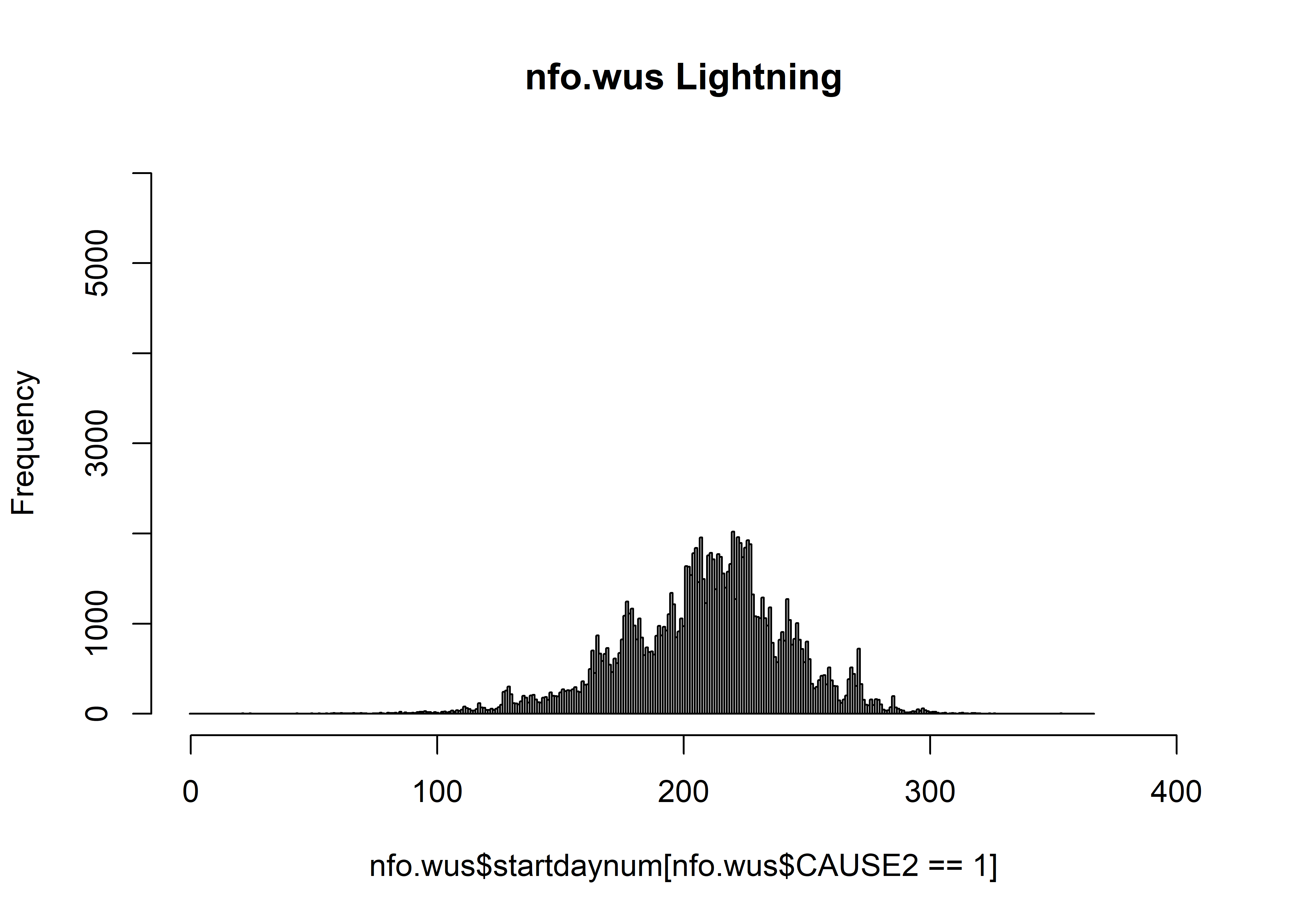
hist(nfo.wus$startdaynum[nfo.wus$CAUSE2==2], breaks=seq(-0.5,366.5,by=1), freq=-TRUE,
  xlim=c(0,400), ylim=c(0,6000), main="nfo.wus Human")